
Welcome to Access 2016: Analyzing & Modifying Data with Queries.
You should have already attended Access 2016: Structuring & Relating Data or have the equivalent skills. Specifically, you should be able to:
This workshop introduces a broad range of features available in Microsoft Access queries and provides hands-on practice on how to:
To complete this workshop successfully, you will be provided with:
These materials presume you will begin work from the desktop, and have any required exercise files located in an epclass folder there.
Most of our workshops use exercise files, listed at the bottom of page 5 of the materials. In our computer-equipped classrooms, these files are located in the epclass folder, which should already be on the computer desktop. If you are using our materials in a different location, you may obtain the exercise files and detailed installation instructions from our Web site at:
http://ittraining.iu.edu/downloads/
Once you are logged on and have the needed files in an epclass folder on your desktop, you are ready to proceed with the rest of the workshop.
If you have computer-related questions not answered in these materials, you may look for the answers in the UITS Knowledge Base, located at:
IT Training offers many training options for extending your skills beyond this workshop:
http://ittraining.iu.edu/online/
Today we will be working with a database that contains information for managing student enrollments at the University of the Midwest.
Our database holds accurate and timely information about the departments, faculty, courses, students, and their enrollments. This information is of little value to us unless we are able to analyze the information and answer questions about it. To examine just the information that we want and to relate it in a meaningful manner, we rely on the use of queries within Access.
We will query the University of the Midwest database to retrieve customized data sets and summarized data sets. We need to be able to see things like which classes students are taking, who is teaching the classes, and where classes are being held. Access queries will help us to sort, filter, summarize, analyze, update, append, and delete the information in our tables.
Let's look at the University of the Midwest database we will use in today's workshop. We will launch Access and then open and explore the database.
Step 1.Launch Access.
Step 2.To begin opening an existing database, in the left pane,
Click Open Other Files
Step 3.To continue,
Click
When the dialog box opens, it lists a default location from where the file will be opened. All of our exercise files are contained in the epclass folder, located on the desktop. We'll want to change our location to this folder.
We will start at the desktop, since our exercise file folder, epclass, is located there.
Step 1.To move to the desktop,
Click
Step 2.To open the epclass folder,
Double-Click
Step 3.To open the correct folder,
Double-Click the Access_AMD folder
Step 4.To open the database file,
Double-Click UofMW.accdb
Step 5.To enable the content,
Click 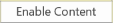
NOTE: Once a file has been opened and enabled from a specific location, Access will consider this location a trusted source and will not show this warning again. For more information regarding trusted documents, refer to the Access online Help documentation.
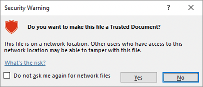
Step 6.To make the file a trusted document, if necessary,
Click 
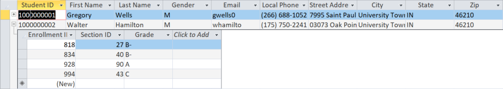
There are twelve tables in the University of the Midwest database: tblCourses, tblDepartments, tblEnrollments, tblFaculty, tblGradeScale, tblLocations, tblMeetingTimes, tblMeetingDays, tblRoles, tblSections, tblSectionsInstructors, and tblStudents. Let's take a moment to look at some of these tables so we have a clear idea of what information they contain. In particular, we will look at the tables we added between Access 2016: Structuring & Relating Data and today's workshop.
Step 1.To view the Students table, in the Navigation pane,
Double-Click tblStudents
Step 2.To view a subdatasheet, next to any record,
Click 
NOTE: If a table is on the "one" side of multiple relationships, instead of seeing a subdatasheet, the Insert SubDataSheet dialog will open. This dialog box allows you to pick what data you want to see in the subdatasheet. To learn more about subdatasheets see:
Step 3.To open the Enrollments table,
Double-Click tblEnrollments
Step 4.To open the Grade Scale table,
Double-Click tblGradeScale
Step 5.To open the Locations table,
Double-Click tblLocations
Step 6.To open the Meeting Days table,
Double-Click tblMeetingDays
Step 7.To open the Meeting Times table,
Double-Click tblMeetingTimes
Step 8.To close all the tables,
Right-Click any tab, Click Close All
The structure of the University of the Midwest database includes tables that allow us to track information about the classes offered at the University of the Midwest. Because all of these table are related, we can ask Access to display in one datasheet information about what department a class is in, who is teaching the class, where the class is located and which students are enrolled in the class.
When working with a relational database, it is important to understand the relationships that exist between the tables. Let's open the Relationships window to view how the tables are related.
Step 1. To see the available database tools, on the Ribbon,
Click the Database Tools tab
Step 2.To view the table relationships for the database, in the Relationships group,
Click 
Table Name |
Related Table |
Join Fields |
tblCourses |
tblSections |
CourseCode = SectionKey |
tblDepartments |
tblCourses |
DeptCode = DeptCode |
tblDepartments |
tblFaculty |
DeptCode = Dept Code |
tblFaculty |
tblSectionsInstructors |
EmployeeID = InstructorID |
tblGradeScale |
tblEnrollments |
LetterGrade = Grade |
tblLocations |
tblDepartments |
LocationID = Office |
tblLocations |
tblFaculty |
LocationID = Office |
tblLocations |
tblSections |
LocationID = Location |
tblMeetingTimes |
tblSections |
MeetingTimeID = MeetingTimeID |
tblMeetingDays |
tblSections |
MeetingDayID = MeetingDayID |
tblRoles |
tblSectionsInstructors |
RoleID = Role |
tblSections |
tblEnrollments |
SectionKey = SectionID |
tblSections |
tblSectionsInstructors |
SectionKey = SectionKey |
tblSections |
tblEnrollments |
student_id = UniversityID |
Step 3.To close the Relationships window,
Right-Click the Relationships tab, Click Close
Since we worked with queries in both Access 2016: The Basics and Access 2016: Structuring & Relating Data, we will start by editing some existing queries. When we are revising these queries, we want to be sure that we don't save over the query we are starting with, so before we start working with criteria, let's make it easier to save queries under a different name.
To make saving queries under a new name easier, we will add the Save As command to the Quick Access toolbar.
NOTE: If you worked through the previous Access workshop materials, the Save As command may already be on the Quick Access toolbar. If so, skip to the next section.
Step 1.To view available commands, on the Quick Access toolbar,
Click  , Click More Commands...
Step 2.To find the Save As command, in the pane on the left, if necessary,
scroll down
Step 3.To add the Save As command,
Double-Click the Save As icon
Step 4.To close the dialog box,
Click 
Now that we have the Save As button on the Quick Access toolbar, let's use it to save the query under a new name.
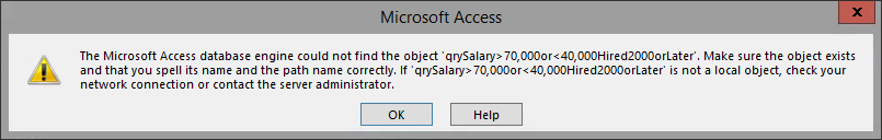
Step 1.To open an existing query,
Double-Click qrySalariesByRank>70,000Hired2000OrLater
2.To switch to Design View,
Click 
Step 3.To save the query, on the Quick Access toolbar,
Click 
Step 4.To name the query, in the Save As dialog box, type:
qrySalary>70,000or<40,000Hired2000orLater,
Click 
We want to alter the query to also see faculty who are making under $40,000 who were hired on or after January 1.
The criteria currently looks like:
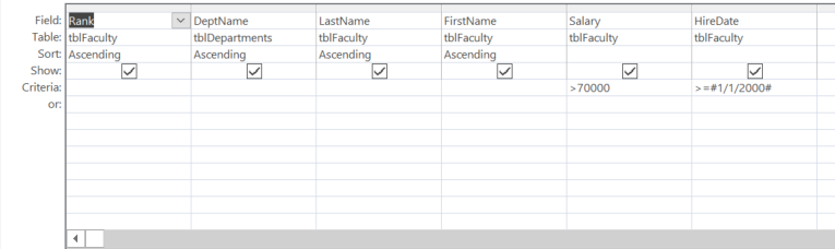
In Access 2016: The Basics, we learned that when we put the criteria in the same row, we are creating an AND query, meaning that both conditions must be true for records to be returned.
In Access 2016: Structuring & Relating Data, we learned that we can use the "or" row to include additional criteria. If we put the <40000 in the Salary field "or" row, we would be creating an OR query that displays people making less than $40,000 regardless of hire date. While we could add the hire date to that second row, there is another way we can create the OR criteria we want in a single row.
We want to combine the criteria for the salary, so we find faculty making more than $70,000 or less than $40,000. In addition to using the grid to create an AND query and an OR query, we can also use the logical operators AND and OR. Logical operators are operators whose results are either true or false.
Step 1.To alter the criteria,
Click after ">70000", type: or <40000 Enter
Step 2.To view the results,
Click
Step 3.To save the changes, press:
Control key+s
Step 4.To close the query,
Right-Click the query tab, Click Close
NOTE: You can also close a query with the keyboard shortcut Control key+w.
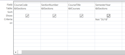
Sometimes it's easier to describe what we want to exclude from our results rather than what we want to include. The NOT logical operator allows us to do this.
Let's revise an existing query to see how NOT works.
Step 1.To open an existing query,
Double-Click qryCoursesAndSectionsSummer18
Step 2.To switch to Design View,
Click
Step 3.To save the query, on the Quick Access toolbar,
Click
Step 4.To name the query, type:
qryCoursesAndSectionsNotSU18 Enter
Step 5.To position the cursor, in the SemesterYear Column,
Click before "SU18"
NOTE: If you have trouble doing this, you can also Click in the SemesterYear criteria row and then press the Home key.
Step 6.To alter the criteria, type:
Not Enter
Step 7.To show the field, in the SemesterYear field,
Click the Show checkbox
8.To view the query,
Click 
Step 9.To save the changes, press:
Control key+s
Step 10.Close the query.
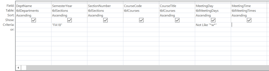
Access allows us to use wildcard characters when we want criteria to be more flexible. The wildcard character in criteria means "anything can go here." The wildcard character is the asterisk (*).
Let's open another query that was created previously and edit it to use wildcards.
Step 1.To open the query,
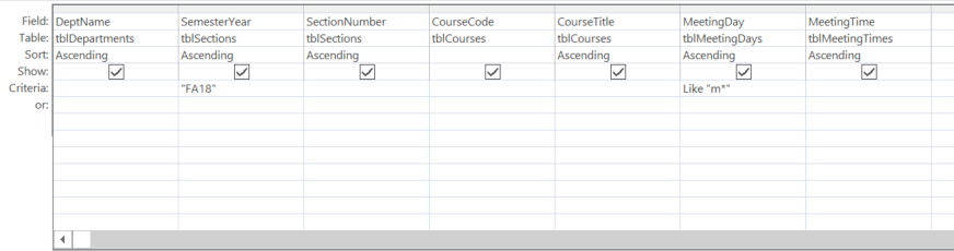
Double-Click qryDeptCoursesFA18NotOnWednesday
Step 2.To go to Design View,
Click
Step 3.To enter the criteria, in the SemesterYear Criteria field, type:
FA18 Enter
Step 4.To enter the new criteria, in the MeetingDay Criteria field, type:
m* Enter
NOTE: The criteria is not case sensitive.
Step 5.To view the query,
Click
Step 6.To return to Design View,
Click
Step 7.To position the cursor,
Click to the left of Like
Step 8.To change the criteria, type:
Not Spacebar Enter
Step 9.To view the query,
Click
Step 10.To return to Design View,
Click
Step 11.To select the current criteria for Meeting Day,
Press & Drag across Like "m*"
Step 12.To change the criteria, type:
*w* Enter
Step 13.To view the query,
Click
Step 14.To save the changes, press:
Control key+s
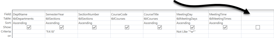
Our query could display the meeting days and meeting times more efficiently. The appearance and readability of this information could be enhanced by combining meeting day and meeting time together in a single field.
So far, we have built queries by selecting fields from tables and adding them to the query design grid. But we are not limited to displaying only fields that already exist in tables. We can create new fields in the design by building an expression. An expression is essentially an equation that describes the information we want to display.
Step 1.To view the query in the query design grid, on the Ribbon,
Click
Step 2.To open a contextual menu, in the query design grid, in the empty column to the right of MeetingTime,
Right-Click in the Field row
3.To open the Expression Builder,
Click Build...
NOTE: If Build is grayed out, click on another field, then right-click the Field row of the empty column again.
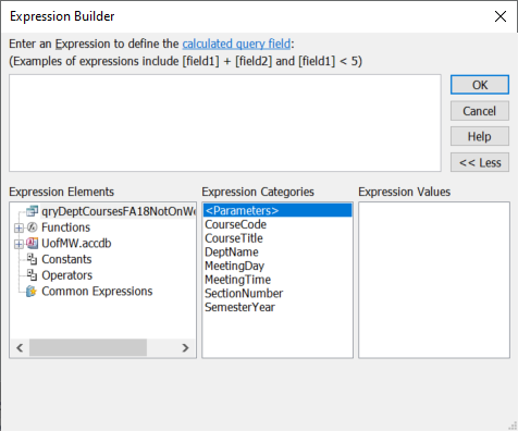
Step 4.To add the MeetingDay field to the expression, in the Expression Categories list,
Double-Click MeetingDay
NOTE: If the name of a field we are using in our expression is included in multiple tables selected as part of the query, we would need to specify both the table name and field name.
Step 5.To add the concatenation operator, after [MeetingDay], type:
+
Step 6.To add a space after [MeetingDay], type:
" "
NOTE: Be sure to type a space between the quotes.
Step 7.To add the concatenation operator, after the quotes, type:
+
![The Expression builder with the start of the expression: [MeetingDay] +" "+](/training/accam/files/pc/img/img_PartialConcatEq.png)
8.To add the MeetingTime field to the expression, in the Expression Categories list,
Double-Click MeetingTime
Step 9.To complete the expression,
Click 
Step 10.To position the cursor to resize the column,
Point to the right border of the Expr1 column
11.To expand the Expr1 column,
Double-Click between the border between the column headers
Step 12.To view the query results, on the Ribbon,
Click
Step 13.To see the Expr1 field, scroll right, if necessary.
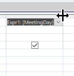
The caption for the column, "Expr1" is generic and is not descriptive of the data. We can change this caption in Design View by placing specific text at the beginning of the expression, followed by a colon.
Let's see how this is done.
Step 1.To return to Design View,
Click
Step 2.To select the current field name, in the concatenated field,
Double-Click Expr1
NOTE: Do not remove the colon since it is needed to separate the caption from the expression.
Step 3.To replace the field label, type:
Meeting Enter
Step 4.To view the query result, on the Ribbon,
Click
Step 5.To see the Meeting field, scroll right, if necessary.
Step 6.To save the changes to the query, press:
Control key+s
We no longer need to see the individual MeetingDay and MeetingTime columns since we now have a column that combines those fields. However, if we delete the MeetingDay column, we would need to keep the criteria. In order to do this, we would need to move the criteria to the new Meeting column. In some cases, if we move the criteria to another column, it may need to be edited and this means extra work for us. Instead, let's hide it from the results and leave the criteria as is.
Step 1.To return to Design View,
Click
Step 2.To hide the Meeting Day field,
Click to deselect the Show field checkbox
Step 3.To begin selecting the MeetingTime column,
Point to the top of the MeetingTime column
Step 4.To select the MeetingTime column, when you see the black down-point arrow,
Click the top of the MeetingTime column
Step 5.To delete the column, press:
Delete key
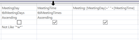
![The selected fields are: DeptName, SemesterYear SectionNumber, CourseCode, CourseTitle, MeetingDay, Meeting Time, and Meeting: [MeetingDay]+" "[MeetingTime]. DeptName, SemesterYear and Section Number are sorted in ascending order. SemesterYear has a critieria of "FA18". MeetingDay has criteria of Not Like "*w*"](/training/accam/files/pc/img/img_qryNotWednesday3.png)
Step 6.To save the query, press:
Control key+s
Step 7.To view the results,
Click
Let's make an additional refinement on our own. Let's combine the SemesterYear and SectionNumber fields into one field called SemYearSect.
Step 1.Edit the query to create a column called SemYearSect that combines the SemesterYear and SectionNumber columns.
2.Save the changes.
Step 3.Close the query.
NOTE: To view a solution for this Challenge Exercise exercise, see Appendix 1: Solution Challenge Exercise: Concatenating Additional Fields on page 104.
In previous examples, you have seen how to enter criteria directly in the query design grid to limit a query's results. Parameter queries provide a more dynamic way to limit results. They prompt the user for the criteria at the time the query is run. The results will match that of the specified criteria.
Suppose we want to limit query results to faculty of a specific department. We could get the desired information by entering criteria in the Criteria field of the query design grid. However, the query would be more flexible if we could enter criteria at the time of execution.
We already have a query that lists all faculty by department. We will begin by modifying that query to include parameter criteria so the user can specify a department as they run the query.
Step 1.To open the query,
Double-Click qryAllFacultyByDept
Step 2.To switch to Design View,
Click
Step 3.To start to save the query with a different name, on the Quick Access toolbar,
Click
Step 4.To name and save the query, type:
qryFacultyDeptRankParams Enter
Step 5.To specify the appropriate criteria, in the DeptName column,
Click the Criteria field,
type: [Enter Department] Enter
NOTE: The square brackets are re quired, and periods are not allowed when entering parameter criteria.
Step 6.To view the query result,
Click
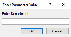
Step 7.To enter a Department name, type:
Biology Enter
NOTE: The text is not case sensitive.
Step 8.To return to Design View,
Click
Step 9.To run this query specifying other departments such as Mathematics or Philosophy,
repeat steps 5 through 7 for other departments
Step 10.To save the changes we made to the query, press:
Control key+s
Suppose we want to see Biology faculty of a certain rank. We will have two criteria parameters. We can place expressions in multiple fields or place multiple expressions in the same field. Access will prompt the user for the first criteria in the query design grid, then prompt for the second criteria. The query then returns data that matches the specified criteria.
Let's make changes to the design of qryFacultyDeptRankParams to allow for an additional parameter.
Step 1.Return to Design View, if necessary,
Step 2.To begin adding a second parameter, in the Rank column,
Click the Criteria field
Step 3.To enter a parameter criteria function, type:
[Enter Rank] Enter
Step 4.To view the query result,
Click
Step 5.To enter a department, type:
Mathematics Enter
Step 6.To enter a rank, type:
Professor Enter
Step 7.To save the changes to the query, press:
Control key+s
Earlier we used the asterisk wildcard in the Criteria field to create more flexible criteria. We saw how to narrow the results to those that meet on a certain day of the week or don't meet on a certain day of the week.
In our example, let's say that we are looking for faculty of a specific department but we don't want to type the whole department name. Because wildcards behave differently when used with parameter criteria, we cannot simply substitute an asterisk for the department. Access would treat the asterisk literally and would search for records where the department included an asterisk.
Access does provide syntax for enabling the use of wildcards in parameter queries. Let's see how to modify the expression in the Criteria field to allow the use of wildcards in the parameter query.
Step 1.To return to Design View,
Click
Step 2.To position the cursor, to the left of the parameter criteria, in the DepartName column,
Click the Criteria field
Step 3.If necessary, to ensure that the cursor is positioned at the beginning of the Criteria field, press:
Home key
Step 4.To use the LIKE operator with your criteria, type:
Like Enter
NOTE: Adding the LIKE keyword is not case sensitive, i.e. "Like" is the same as "like." Access will change the case automatically.
Step 5.To set wildcard criteria for the Rank column,
repeat steps 2 through 4
Step 6.To view the query result,
Click
Step 7.In the dialog box, type:
p* Enter
Step 8.In the dialog box, type:
as* Enter
NOTE: You can also mix and match when using the asterisk. For example, you can look for all of the Mathematics faculty by entering "Mathematics" in the Department prompt and by entering an asterisk in the Rank prompt.
NOTE: The * wildcard character will not return null values (that is, empty fields). To see null values in a parameter criteria query, in Design View, add the text Or Is Null after the parameter. For example: Like [Enter the Rank] Or Is Null.
Step 9.To return to Design View,
Click
Step 10.To save the changes, press:
Control key+s
Queries can be used to search for data where the criteria cover a range of information, like a specific time period or price range. When we want to specify a range, we can combine parameter expressions with operators like this:
>=[Enter a start date] And <[Enter an end date]
In this case >=, <, and And are operators.
Let's try using this method to search for faculty hired within a certain date range.
Step 1.Return to Design View, if necessary.
Step 2.To start to save the query under a new name,
Click
Step 3.To name the new query, type:
qryFacultyHireDateRangeParam Enter
Step 4.To position the cursor,
Click anywhere in the Criteria row
Step 5.To select and delete the criteria, press:
Control key+a, Delete key
Step 6.To add the HireDate field, from the top panel, in tblFaculty,
Double-Click HireDate
Step 7.To open the Zoom window,
Right-Click the HireDate Criteria field, Click Zoom...
NOTE: If Zoom is grayed out, click another field and then right-click the Criteria row of the HireDate column again.
Step 8.To create a parameter query to view faculty hired in a specific date range, type:
>=[Enter a start date] And <[Enter an end date] Enter
Step 9.To view the query result,
Click
Step 10.To enter a start date, type:
1/1/2001 Enter
Step 11.To enter an end date, type:
1/1/2006 Enter
Step 12.To save the changes, press:
Control key+s
Step 13.Close the query.
Let's add parameters to another existing query to allow us to see the professors teaching courses in a specified semester.
Step 1.Open qryCoursesSectionsAndAllFacultySummer18.
Step 2.Switch to Design View.
Step 3.Save it as "qryCoursesSectionsAndAllFacultySemesterParameter."
Step 4.Add the required parameter to the SemesterYear field.
NOTE: If you keep the Or is Null, which is part of the current criteria for SemesterYear, the results will include the faculty for the semester entered and all faculty who are not assigned to teach in any semester. This also means the query can be run with no parameter value entered, which will only show faculty who aren't assigned to teach in any semester.
Step 5.Save and test the query.
Step 6.Close the query.
NOTE: To view a solution for this Challenge Exercise exercise, see Appendix 2: Challenge Exercise: Adding Parameters to a Query on page 104.
Queries can summarize and display information by groups. A group is a collection of related records. A sales database could group all orders by each customer. A property database could group all equipment by manufacturer. Our database could group all faculty by department.
Grouping then allows further analysis of the data. For example, we could total, average, or count some value for each group.
We will create a query that will show the total number of faculty members in each department.
Step 1.To start to create a new query, on the Ribbon,
Click the
Create tab, Click 
Step 2.To add required tables to the query design grid, in the Show Table dialog box,
Double-Click tblDepartments,
Double-Click tblFaculty
Step 3.To close the Show Table dialog box,
Click 
Step 4.To place the DeptName field in the query, from tblDepartments,
Double-Click DeptName
Step 5.To add the EmployeeID field to the query, from tblFaculty,
Double-Click EmployeeID
Step 6.To turn on the Totals function, in the Show/Hide group of the Ribbon's Design tab,
Click 
Let's look at the ways Totals can summarize our data. Access allows the choice of a number of options and aggregate functions in the Total row. Aggregate calculations are predefined operations performed on groups of records. They can provide totals, counts, averages, and other information about field values in all records or in groups of records. Following is a list of the available aggregate functions:
Function |
Purpose |
Sum |
Totals the values for each group |
Avg |
Averages the values for each group |
Min |
Returns the lowest value in each group |
Max |
Returns the highest value in each group |
Count |
Returns the number of items in each group |
StDev |
Returns the standard deviation for each group |
Var |
Returns the variance for each group |
First |
Returns the first value in the group |
Last |
Returns the last value in the group |
Expression |
Returns a calculation based on an aggregate function |
Where |
Specifies criteria to select specific records |
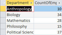
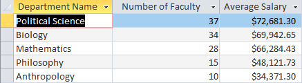
The Count function returns the number of unique items in each group. So in our example, if we group by department and choose the Count function in the EmployeeID column, the query will group all faculty by their department and count them. Let's use the Count function to count the employee IDs in each group.
Step 1.To see the various functions,
Click the EmployeeID Total row
Step 2.To see the available aggregate functions, in the Employee ID Total row,
Click 
Step 3.To select the Count function, on the drop-down list,
Click Count
Step 4.To view the query result,
Click
NOTE: The departments are in alphabetical order, but not because we sorted them. They are actually in order by department code, which is the structure of the underlying data.
Step 5.To see the entire label in the first column,
expand the first column of the Datasheet
Step 6.To see the entire label in the second column,
expand the second column of the Datasheet
Step 7.To return to Design View,
Click
Step 8.To position your cursor properly, in the query design grid at the bottom of the screen,
Click before the text "EmployeeID"
Step 9.To change the label, for the second column, type:
Number of Faculty: Enter
NOTE: Remember, you have to include the colon as the separator between the caption and field name, but the colon will not be displayed in the field.
Step 10.To see the result of changing the label, on the Ribbon,
Click
Step 11.To save the query, press:
Control key+s,
type: qryFacultySalaryAggFunctions Enter
Another piece of data that would be useful to include is the average of faculty salaries in each department. We can modify qryFacultySalaryAggFunctionsto retrieve this information.
Step 1.To return to Design View,
Click
Step 2.To add the Salary field, from the tblFaculty field list,
scroll down, Double-Click Salary
Step 3.To select the field to be changed,
Click the Salary field Total row
Step 4.To select the Avg function,
Click , Click
Avg
Step 5.To position the cursor properly, in the Salary field,
Click before "Salary"
Step 6.To rename the field, type:
Average Salary: Enter
Step 7.To begin to change the sort order,
Click the Salary Sort row
Step 8.To change the sort order to descending, type:
d
Step 9.To view the query result, on the Ribbon,
Click
Step 10.Expand any columns, if necessary.
11.To save the changes to the query, press:
Control key+s
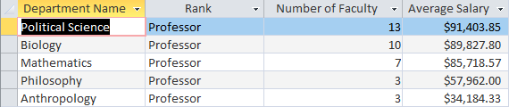
A query can be grouped by multiple fields. For example, a query could group three fields to identify an employee: EmployeeID, LastName, and FirstName. In the totals row, all three of these columns would be set to the Group By option.
Next we will add the Rank field to this query in order to view the summary for each rank of faculty.
Step 1.To switch to Design View,
Click
Step 2.To add the Rank field to the grid, starting in tblFaculty, in the top panel,
Press & Drag Rank until it is on top of the Number of Faculty: EmployeeID field
Step 3.To list the departments in alphabetic order, in the DeptName field,
Click the Sort field, Type: a
Step 4.To switch to Datasheet View,
Click
We could expand the usefulness of this query by including a parameter to allow the user to specify a rank. The resulting summary would then show the total salaries for all professors, all assistant professors, or whatever rank was entered. We will add criteria in the Rank column and enter the expression that will prompt the user for a rank of faculty when the query is executed.
Step 1.To return to Design View,
Click
Step 2.To set the criteria to make this a parameter query, in the Criteria row under Rank, type:
Like [Enter Rank] Enter
Step 3.To switch to Datasheet View,
Click
Step 4.To supply a rank for the parameter, type:
Prof* Enter
5.To save the change to the query, press:
Control key+s
Step 6.Close the query.
You have seen how aggregate calculations are created in queries and that they summarize data for a group of records. You can also make calculations on a row-by-row basis, using calculated fields. Calculated fields contain customized expressions. The concatenated Meeting field that we made earlier is a simple example of a calculated field. Calculated fields are created and recomputed each time a query is executed.
In the next query, our eventual task is to generate the GPA for each of the students. To determine this, we will need to use both calculated fields and aggregate functions.
GPA values are calculated by the following formula:
Sum(PointValue*CreditHours)/Sum(CreditHours)
We'll create our complex calculated field by combining multiple simpler calculations.
The first calculation we need is the weighted grade, by multiplying the PointValue of the student's grade by CreditHours available for the course.
Let's begin by opening a query that is partially completed.
Step 1.To open the query,
Double-Click qryGPACalc
Step 2.To switch to Design View,
Click
Step 3.To open a contextual menu, in the query design grid, in the empty column to the right of Credit Hours,
Right-Click the Field row
Step 4.To launch the Expression Builder,
Click Build...
NOTE: If Build is grayed out, click another field, then right-click the field row of the empty column again.
Step 5.To add the first value to the expression, in the Expression Categories field,
Double-Click PointValue
Step 6.To add the multiplication operator, type:
*
Step 7.To add the next value to the expression,
Double-Click CreditHours
Step 8.To close the Expression Builder,
Click
Step 9.To replace the field label, in the query design grid,
Double-Click "Expr1", type: Weighted Enter
Step 10.To view the query result,
Click
Step 11.To widen the column, on the right border of the Weighted column,
Double-Click 
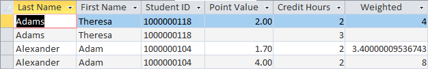
NOTE: Each student's records may appear in a different order.
If we examine the enrollments data, we can see the difference can be accounted for by the records where no grade was reported. Why don't these records appear in this dynaset? It's due to the join properties of the relationship between tblGradeScale and tblEnrollments:
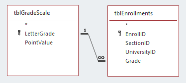
The relationship between the tblEnrollments and tblGradeScale tables is established using the Grade field, from tblEnrollments, and the LetterGrade field, from tblGradeScale, as we see in the previous diagram. This relationship is using the join type called inner join. In Access 2016: Structuring & Relating Data, we learned that this type of join only returns the records where the data exists on both sides of the relationship. This means when the Grade field is empty, there isn't a match between the two tables, and these records are excluded from our results.
So what are the records that appear in our results that don't have a PointValue? These are students who received an incomplete in a course. If a student is given an incomplete for a course, the instructor records the grade as an "I." Since the grade "I" appears in both tblEnrollments and tblGradeScale, these records are included in the results. However, there is no point value associated with I grades in tblGradeScale, and if we don't exclude them from the GPA calculation, the results of our calculation will be inaccurate.
Let's exclude any records where the PointValue column is blank.
Step 1.To return to Design View,
Click
Step 2.To specify the appropriate criteria, in the PointValue column,
Click the Criteria field, type: Is Not Null Enter
Step 3.To view the query result,
Click
Step 4.To save the changes to this query, press:
Control key+s
Now that we have eliminated incomplete grades, we need to sum together the rest of the records for each student. Remember, the Totals function allows us to use predefined operations, including Sum, on groups of records.
Remember the equation for GPA is:
Sum(PointValue*CreditHours)/Sum(CreditHours)
We created the Weighted calculated column that shows the results of multiplying the PointValue by the Credit Hours. So the equation we are working with at this point is:
Sum(Weighted)/Sum(CreditHours)
What we need to do now is to sum the rows that are for the same student together. So if a student has grades in three classes, the values are added together to give us a sum value for each student's Weighted and CreditHours columns. This will give us the total weighted points the student has earned and the total credit hours each student has taken.
Step 1.To return to Design View,
Click
Step 2.To turn on the Totals function, in the Show/Hide group of the Ribbon's Design tab,
Click
Step 3.To select the CreditHours Total row,
Click the CreditHours Total row
Step 4.To set the function to sum, in the CreditHours Total row,
Click , Click
Sum
Step 5.To rename the CreditHours field,
Click before
"CreditHours",
type: Total Credit Hours: Enter
Step 6.To set the Weighted aggregate calculation,
Click the
Weighted Total field, Click , Click
Sum
Step 7.To view the query result,
Click
Step 8.To return to Design View,
Click
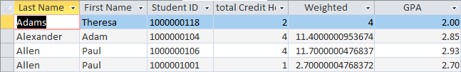
![The selected fields are last_name, first_name, student_id, PointValue, Total Credit Hours: Credit Hours and Weighted: [PointValue] * [CreditHours]. The Total row is now appearing. The last_name, first_name, student_id, and PointValue have Group By in their Total field. PointValue has criteria of Is Not Null. The Total Credit Hours: Credit Hours and Weighted: [PointValue] * [CreditHours] have Sum in their Total row.](/training/accam/files/pc/img/img_qryGPACalc2.png)
NOTE: Setting the Total field to Where isn't required if you do want to group by that field. For example, in the previous query, we added parameter criteria for Rank and also grouped by Rank, so we used Group By.
Step 9.To change the Total row setting for PointValue,
Click the
Total row, Click , Click
Where
Step 10.To view the query result,
Click
Step 11.To save the changes we have made, press:
Control key+s
Now that we have the sum total for the values in the Weighted and Total Credit Hours fields for each student, we need to use those values to create another calculated field to divide the value of the Weighted column by the value of the Total Credit Hours column.
Step 1.To return to Design View,
Click
Step 2.To open a contextual menu, in the query design grid, in the empty column to the right of Weighted,
Right-Click the Field row
Step 3.To launch the Expression Builder,
Click Build...
NOTE: If Build is grayed out, click another field, then right-click the field row of the empty column again.
Step 4.To start the expression, in Expression Categories list,
Double-Click Weighted
NOTE: If you don't see Weighted, close the Expression Builder and save the query. Then reopen the Expression Builder.
Step 5.To add the division symbol, type:
/
Step 6.To finish the expression, in Expression Categories list,
Double-Click Total Credit Hours
NOTE: If you don't see Total Credit Hours, close the Expression Builder and save the query. Then reopen the Expression Builder.
Step 7.To close the Expression Builder,
Click
Step 8.To replace the field label,
Double-Click Expr1, Type: GPA Enter
![Subqueries cannot be used in the expression (Sum([Weighted]/[Total Credit Hours])).](/training/accam/files/pc/img/dbox_SubqueriesWarning.png)
Step 9.To set the function to Expression, in the Total row under the GPA column,
Click , Click
Expression
Step 10.To view the query result,
Click
Step 11.Expand the GPA column, if necessary.
We would like the GPA to have just two decimal places. Let's fix the formatting of the GPA.
Step 1.To return to Design View,
Click
Step 2.To see the properties for the GPA column, if necessary,
Click an
empty part of the column, Click 
Step 3.To set the format for the field, in the Property Sheet,
Click the
empty space next to Format,
Click , Click
Fixed
Step 4.To set the number of decimals, in the Decimal Places row, type:
2
Step 5.To view the query result,
Click
We needed the Total Credit Hours and Weighted columns to calculate the GPA, however we don't really need to see them in the query results. It would seem that you could just deselect the Show cbeckbox in the query design for these two columns. However, if we tried this, when we viewed the query, parameter dialogs would appear, prompting us for values for both Total Credit Hours and Weighted. Earlier, we mentioned that Access shows parameter dialogs whenever it doesn't understand an object or expression. Deselecting the Show checkbox actually alters the SQL used in the query. In our case, this would mean Access wouldn't know what the values of Weighted and Total Credit Hours were for the GPA calculation.
There is a way around this: we can hide the columns in Datasheet View. Hiding values in Datasheet View doesn't alter the SQL; instead it sets their width to 0. This means they are hidden from display, but the SQL statement does not change.
Step 1.To select both the columns,
Point to the Total Credits column heading, Press & Drag over to Weighted
Step 2.To hide the columns, on the Home tab of the Ribbon, in the Records group,
Click  , Click
Hide Fields
, Click
Hide Fields
Step 3.To save the changes to the query, press:
Control key+s
Structured Query Language (SQL) is a standardized data query language that was created for the purpose of working with databases. For those intending to work with server databases such as Oracle and SQL Server, knowledge of SQL is essential. One subset of SQL can be used to form statements that create, retrieve, update, or delete data.
Access automatically translates a query into the Access version of SQL, but it is not necessary to know SQL in order to create queries in Access. Knowing SQL, however, could enable you to customize more powerful Access queries. Also, when working with forms and reports in Access, there will be times when you are asked to save changes to the SQL statement. By exploring the SQL View now, you will be more familiar with the terminology.
We can easily view the SQL version of queries we create. Let's explore the SQL View of this query.
Step 1.To select a different view of this query, on the Ribbon,
Click  , Click SQL View
Step 2.To deselect the text,
Click anywhere in the window
![SELECT tblStudents.last_name, tblStudents.first_name, tblStudents.student_id, Sum(tblCourses.CreditHours) AS [Available Credits], Sum([PointValue]*[CreditHours]) AS Weighted, [Weighted]/[Available Credits] AS GPA FROM tblStudents INNER JOIN ((tblCourses INNER JOIN tblSections ON tblCourses.CourseCode = tblSections.CourseCode) INNER JOIN (tblGradeScale INNER JOIN tblEnrollments ON tblGradeScale.LetterGrade = tblEnrollments.Grade) ON tblSections.SectionKey = tblEnrollments.SectionID) ON tblStudents.student_id = tblEnrollments.UniversityID WHERE (((tblEnrollments.Grade)<>"i")) GROUP BY tblStudents.last_name, tblStudents.first_name, tblStudents.student_id ORDER BY tblStudents.last_name, tblStudents.first_name, tblStudents.student_id;](/training/accam/files/pc/img/img_SQLstatement.png)
NOTE: For more information on Structured Query Language, consider taking the workshops: SQL: Data Retrieval and SQL: Advanced Data Retrieval and Data Modification.
Step 3.Close the query.
Access offers another tool for summarizing data—the Crosstabquery. A Crosstab query uses a function to calculate data that is grouped by two types of information—one down the left side of the datasheet and another across the top. The specified calculation is performed at each row-column intersection resulting in a spreadsheet-like summary of the objects specified in the row and column headers. Crosstab queries allow the display of data in a format that facilitates analysis of grouped and calculated data.
Crosstab queries have at least three fields:
The following Crosstab query example from a car sales database demonstrates these fields:
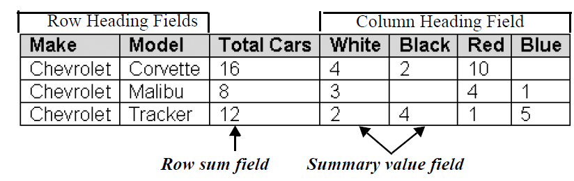
NOTE: The row sum field that you see in the previous diagram, which totals all calculations for the row, is optional.
Since Crosstab queries are a more advanced type of query, there is a wizard for creating them, however the Crosstab Query Wizard has limitations that make it less than ideal. The main limitation is that queries created using it need to be based on a single table or query. If a Crosstab query requires fields from multiple tables, a query that contains the needed information must first be created, and then that query can be used with the Crosstab Query Wizard.
In the next exercise, we will create a Crosstab query that pulls data from multiple tables. Rather than pull that data together into a query and use it as the data source for the wizard, we will create a Crosstab query in Design View.
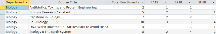
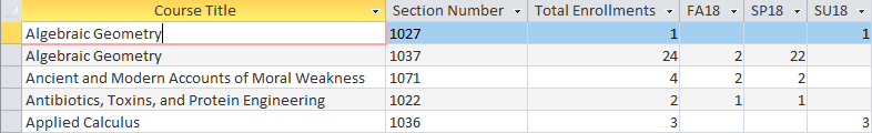
Let's create a Crosstab query in Design View that will show departments, courses and enrollments. The row headings will be DeptName and CourseTitle. The column heading will be SemesterYear. In the intersecting cells, a count of EnrollID will show students enrolled in each semester/year.
The query results will look like this:
Let's create this Crosstab query.
Step 1.To begin creating a new query, on the Ribbon,
Click the
Create tab, Click
Step 2.To add the tables we want to the query design window,
Double-Click tblEnrollments,
tblSections,
tblCourses, tblDepartments
Step 3.Close the Show Table dialog box.
Step 4.To save this query, press:
Control key+s, Type: qxtbEnrollmentsByDepartmentsAndCourses Enter
NOTE: The "qxtb" is the standard Access naming convention prefix for Crosstab queries.
By default, Access assumes new queries will be Select queries and the query design grid accommodates that query type. The first step in building a Crosstab query is to change the query type from the default Select Query to Crosstab Query.
Step 1.To define the query type, in the Query Type group on the Ribbon,
Click 
Step 2.To add the first row heading field to the query, in tblDepartments,
Double-Click DeptName
Step 3.To add the second row heading field to the query, in tblCourses:
Double-Click CourseTitle
Step 4.To position the cursor, in the DeptName column,
Click the Crosstab cell
Step 5.To designate this field as a row heading,
Click , Click
Row Heading
Step 6.To designate the CourseTitle field as a row heading, in the CourseTitle column,
Click the
Crosstab cell, Click , Click
Row Heading
Step 7.To add the SemesterYear field to the query, in the tblSections field list,
Double-Click SemesterYear
Step 8.To designate this new field as a column heading, in the SemesterYear column,
Click the
Crosstab cell,
Click , Click
Column Heading
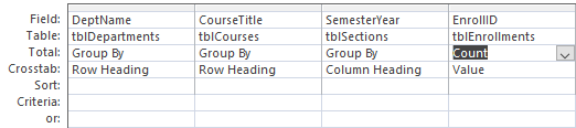
Step 9.To add the EnrollID field to the query design grid, in the tblEnrollments field list,
Double-Click EnrollID
Step 10.To set this field to perform the Value calculation, in the EnrollID column,
Click the
Crosstab cell, Click , Click
Value
Step 11.To set the calculation to Count, in the EnrollID field,
Click the
Total cell, Click , Click
Count
We would like to have a total column in our Crosstab query. Let's see how to create a total column.
Since we are again counting number of enrollments in the total column, the EnrollID field is the field to use. Let's add the EnrollID field to the query design grid for a second time.
Step 1.To add the EnrollID field to the query a second time, from the field list,
Double-Click EnrollID
Step 2.To set the calculation to be performed, in the second EnrollID field,
Click the
Total cell, Click , Click
Count
Step 3.To define this field's purpose, in the second EnrollID field,
Click the
Crosstab cell, Click , Click
Row Heading
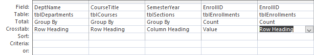
Step 4.To set the caption,
Click at the beginning of the second EnrollID field, type: Total Enrollments:, press: Enter
Step 5.To see the query results, on the Ribbon,
Click
Step 6.Expand the column headings.
7.To save the query, press:
Control key+s
Step 8.Close the query.
Let's create another Crosstab query that lets us see the data in a different way. We want to see how many students are enrolled in the sections of courses each semester.
Step 1.Create a new query called:
qxtbEnrollmentsByCourseAndSection
Step 2.Add the row headings.
Step 3.Add a column heading.
Step 4.Add a value.
Step 5.Add a total column.
6.Close the Crosstab query.
NOTE: To view a solution for this Challenge Exercise exercise, see Appendix 3: Challenge Exercise: Building Another Crosstab Query on page 105.
Up to this point in the workshop, we have built Select queries, Totals, and Crosstab queries, which create dynasets that show the most current information in the selected fields and tables. The results of a query may be different at any given time, depending upon the underlying data.
Another type of query is the Action query, which makes changes to the underlying data. Instead of just viewing data, Action queries can easily alter data by updating field values, deleting records, or adding new records. It is easy to see that Action queries can be very powerful tools in performing global data management operations on one or more tables at once. At the same time, they can also be dangerous since an erroneously written query can make incorrect changes to thousands of records. We will keep this in mind and learn how to protect our data as we explore Action queries.
Select queries will serve users' needs most of the time. That's why they are the default query type. However, sometimes Action queries are needed.
The following table lists the different types of Action queries in Access:
Action Query Type |
Description |
Make Table |
Creates a new table which contains selected data |
Update |
Updates table data according to query specifications |
Append |
Appends data from one table to another according to query specifications |
Delete |
Deletes records according to query specifications |
In today's exercises, we will create these Action queries:
Because Action queries modify data, they are very powerful. However, if the specifications or expressions used to design an Action query are incorrect, we are left with bad data after the Action query is run. Therefore, we should always make copies or backups of the tables before running an Action query on them.
In our Action query exercises today, we will make changes to tblLocations, tblCourses, and tblFaculty. Let's make backups of these tables before we start building Action queries.
Step 1.To select the tables,
Click tblCourses,
press: Control key and Click tblFaculty,
press: Control key and Click tblLocations
Step 2.To make a copy of the tables, press:
Control key+c
Step 3.To paste the copy the tables, press:
Control key+v
Step 4.To name and create the new table for courses, type:
zzBackup_tblCoursesToday'sDate Enter
Step 5.To name the table, type:
zzBackup_tblFacultyToday'sDate Enter
Step 6.To name the table, type:
zzBackup_tblLocationsToday'sDate Enter
Let's open the tables and verify that the copy happened correctly.
Step 1.To open the tables,
Double-Click tblCourses, tblFaculty, tblLocations, zzBackup_tblCoursesToday'sDate, zzBackup_tblFacultyToday'sDate, zzBackup_tblLocationsToday'sDate
Step 2.To view tblCourses,
Click the tblCourses tab
Step 3.To view the backup of tblCourses,
Click the zzBackup_tblCoursesToday'sDate tab
Step 4.To verify that both tblFaculty and its backup have 124 records,
repeat steps 2 and 3
Step 5.To verify that both tblLocations and its backup have 124 records,
repeat steps 2 and 3
Step 6.To close all tables,
Right-Click any tab, Click Close All
The Make Table query is a select query that pulls data from a database based on certain criteria, and then saves that data into a new table. The new tables that result from Make Table queries can be used for different purposes. For example, a table can be used to hold inactive records for a specific point in time and then used as the basis for historical reports about that period. The Make Table query is also useful for making some information in an existing table available to other users without exposing all fields of the table. New tables can also enhance the performance of very complex queries based on multiple tables. The table becomes the record source for forms or reports, and the query doesn't have to run each time those objects are opened.
As we pointed out earlier, the Locations table was added to the database after the Access 2016: Structuring & Relating Data workshop. Let's take a look at the data currently stored in the Locations table.
Step 1.To open the table,
Double-Click tblLocations
Step 2.Close tblLocations.
Step 3.To begin creating a new query, on the Ribbon,
Click the
Create tab, Click
Step 4.To select the table we need to create this query, in the Show Table window,
Double-Click tblLocations
Step 5.Close the Show Table dialog box.
Step 6.To add the needed fields to the grid,
scroll down as needed, Double-Click the BuildingCode, BuildingName, StreetAddress, City, State, and Zip fields
Step 7.To preview the query, on the Ribbon,
Click
Step 8.To return to Design View,
Click
Step 9.To make the query the selected object,
Click the empty gray area in the top half of the Query window
Step 10.To view the query properties, in the Show/Hide group of the Design tab, if necessary,
Click
NOTE: If you only see a few properties, click somewhere in the top half of the query workspace, outside the tblLocations field list.
Step 11.To set the Unique Values option, in the Unique Values field,
Double-Click No
Step 12.To see the results of the query, on the Ribbon,
Click
We need to tell Access that we want this to be a Make Table query instead of the default Select query type.
Step 1.To return to Design View,
Click
Step 2.To designate the query as a Make Table query, on the Design tab of the Ribbon, in the Query Type group,
Click 
Step 3.To name the table, type:
tblBuildings Enter
Step 4.To run the Make Table query, on the Ribbon,
Click 
Step 5.To complete the creation of the new table,
Click 
Step 6.To close the query without saving changes,
Right-Click the
query tab, Click Close, Click 
While we have created our new table called tblBuildings, it does not yet have a primary key nor is it related to any other tables. There must be a primary key assigned before we can establish relationships to other tables.
Let's assign a primary key to the Buildings table.
Step 1.To open tblBuildings in Design View, in the Navigation Pane,
Right-Click tblBuildings, Click Design View
Step 2.To select the BuildingCode field, if necessary,
Click the BuildingCode field
Step 3.To set the BuildingCode field as the primary key, on the Ribbon, in the Tools group,
Click 
Step 4.To save the changes to the table design, press:
Control key+s
Step 5.Close the table.
The Buildings table needs to be related to the Locations table.
Let's relate the Locations and Buildings tables.
Step 1.To access the Relationships window, on the Ribbon,
Click the
Database Tools tab, Click
Step 2.To start to add a table, on the Ribbon, in the Relationships group,
Click 
Step 3.To add the Buildings table to the Relationships window,
Double-Click tblBuildings
Step 4.To close the Show Table dialog box,
Click
Step 5.To position tblBuildings closer to the tblLocations table,
Press & Drag the tblBuildings title bar and move it to the left of tblLocations
Step 6.To expand the field list, if necessary,
Press & Drag the bottom border of the field list
Step 7.To create a one-to-many relationship, from tblBuildings to tblLocations,
Press & Drag BuildingCode in tblBuildings onto BuildingCode in tblLocations
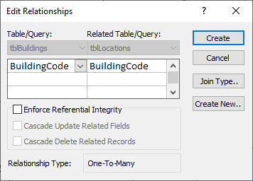
8.To enforce referential integrity,
Click the "Enforce Referential Integrity" checkbox
Step 9.To cascade update related fields,
Click the "Cascade Update Related Fields" checkbox
Step 10.To create the relationship,
Click 
Step 11.To close the Relationships window,
Right-Click the Relationships tab, Click Close
Step 12.To save the layout changes,
Click
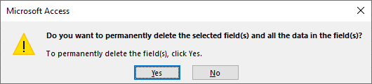
When we used the Make Table query to create the Buildings table, the data also remained in the Locations table. We would like to remove the duplicate information. It might seem that a Delete query would be used to do this but that is not the case. Delete queries allow us to delete rows of data, not fields.
Let's remove the duplicate fields,
Step 1.To open the Locations table, in the Navigation pane,
Right-Click tblLocations, Click Design View
Step 2.To select BuildingName,
Click the gray box to the left of BuildingName
Step 3.To select the rest of the duplicate columns,
Shift key+Click the gray box to the left of Zip
Step 4.To start to delete the columns, press:
Delete key
Step 5.To finish deleting the fields,
Click 
Step 6.To save the changes to the design, press:
Control key+s
Step 7.Close the table.
The Append query allows records to be restored to or added to an existing table. Append queries allow us to add new records to the database without going through time consuming data entry. This approach can be an alternative to bringing data directly into an existing table using the import tools, especially when there are mismatches between existing fields and those imported.
The English department at the University of the Midwest is going to start using the database we have been creating. We already added the English department to tblDepartments. The English department has been keeping the list of their courses in an excel file. We want to add these records to tblCourses. Since the structure of the spreadsheet doesn't match our table structure, the spreadsheet's data needs to be imported into the database and placed in a new table; then we can append the data from that table into our existing Employees table.
Step 1.To begin importing data, on the Ribbon,
Click the External Data tab
Step 2.To import an Excel file, in the Import & Link group,
Click 
Step 3.To begin finding the correct file, to right of the File name text box,
Click 
Step 4.Navigate to the Access_AMD subfolder within the epclass folder.
Step 5.To select the spreadsheet file to import,
Double-Click EngCourses.xlsx
Step 6.To continue, if necessary,
Click the
"Import the source data into a new table in the current database"
radio button, Click
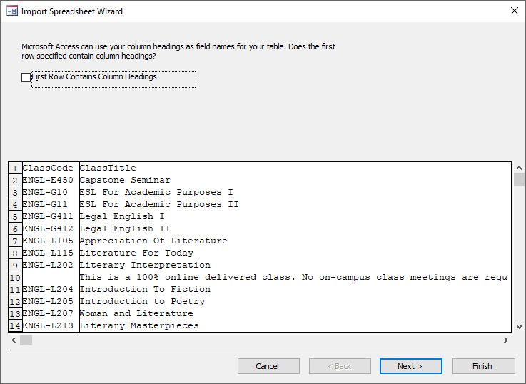
Step 7.To select the First Row Contains Column Headings option,
Click the "First Row Contains Column Headings" checkbox
Step 8.To finish the wizard,
Click 
Step 9.To close the dialog box without saving the import steps,
Click
Before we append the data to the Courses table, we should review what we imported to be sure the import went as expected.
Let's open the table.
Step 1.To open the new table, in the Navigation pane,
Double-Click EngCourses
Step 2.To expand the ClassTitle column,
Point between the ClassTitle and Description headings, Double-Click to expand the ClassTitle column
Step 3.To start to close the table,
Right-Click EngCourses tab, Click Close
Step 4.To skip saving the changes to the layout of the table,
Click
It is generally a bad practice to delete data. Once the data is gone, it may not be able to be recovered.
Let's say a student had graduated and left the University of the Midwest. If we deleted that student and referential integrity wasn't enforced, we would then have orphan records for that student's enrollments in tblEnrollments, and we would only have a student ID with no other information about that student in our database.
On the other hand, if referential integrity was enforced, to delete the student, we would need to turn on Cascade Delete Related Records for the relationship between tblStudents and tblEnrollments. If we deleted the student at this point, we would remove both the student record and the records of any courses the student enrolled in, including their grades. This would delete important historical enrollment and grade information.
In either case, if the student wanted a transcript of their course at the university at some time in the future, it would be very difficult, if not impossible, to provide this information to the student.
An alternative to deleting data is to include a Yes/No field indicating whether the record is active or inactive. This means that the data is still available for us to refer back to. The one real downside to having an active field is that we need to remember to take this field into account when writing queries.
In the table we just created we don't have to worry about relationships as it isn't yet related to other tables. It also is one of those rare instances where using a Delete query makes sense. A Delete query removes entire records from the database. We can delete the data we imported because it's new, and we don't want the records we are removing to ever become integrated into our database. Let's use a Delete query to remove the stray comment rows.
Step 1.To start creating a new query, on the Ribbon,
Click the
Create tab, Click
Step 2.To add the EngCourses table to the design, in the Show Table dialog box,
Double-Click EngCourses, Click Close
Step 3.To select all the fields, in the EngCourses field list
Double-Click 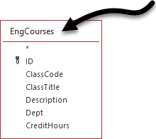
Step 4.To place all the fields on the query design grid, with all the fields selected,
Press & Drag any field to the query design grid
NOTE: If you Double-Click the asterisk, all fields will display in the query dataset, but the fields won't show up individually on the query design grid.
Step 5.To change the query type, on the Design tab, in the Query Type group,
Click 
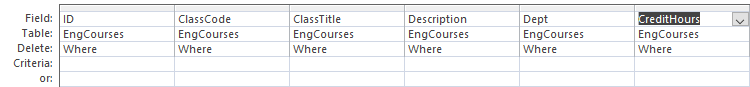
Step 6.To add the Criteria to select the notes, in the ClassCode field,
Click the Criteria cell, Type: Is Null
Step 7.To view the records to be deleted,
Click
Step 8.To return to Design View,
Click
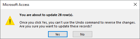
Step 9.To run the Delete query,
Click
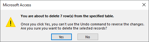
Step 10.To continue the delete process,
Click
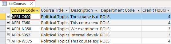
While Access showed us a message confirming the deletion, we want to be sure that the data we expected was deleted. Let's take a look at EngCourses to be sure the rows were deleted.
Step 1.To open the EngCourses table,
Double-Click EngCourses
Step 2.Close the table.
Now that we have only the data we want in the EngCourses table, we can change our query to an Append query to allow us to add the remaining records to tblCourses.
One thing we need to deal with when appending data from one table to another is the differences in how the tables are structured. Before we try to append the records from EngCourses to tblCourses, we need to study the structure of the two tables. Are their fields compatible?
These images compare fields in both tables:
We can readily identify some potential roadblocks to the append action. The table EngCourses has:
As the graphic shows, the two tables that will be used for the Append query do not have matching fields. Let's proceed and see how Access helps us to deal with these issues using the Append query.
Step 1.To switch to the Query Tools Design tab, on the Ribbon, under the Query Tools contextual tab,
Click the Design tab
Step 2.To change the query type, on the Design tab, in the Query Type group,
Click 
Step 3.To select the table you want to append to, on the drop-down list,
Click , Click
tblCourses
Step 4.To confirm your settings,
Click
Step 5.To remove the criteria,
Press & Drag across "Is Null", press: Delete key
Notice the Append To row that has been added to the query design grid. Where Access recognizes a match between field names, the destination field name is filled in. In the other fields, ID, ClassCode, ClassTitle, and Dept, Access left the Append To row blank. It needs help to identify the destination field.
Step 1.To start identifying the destination field for the ClassCode column,
Click the "Append To" field in the ClassCode column
Step 2.To select the matching field,
Click , Click
CourseCode Tab key
Step 3.To identify a match for the ClassTitle field, in the Append To row:
Click , Click
CourseTitle, press: Tab key
Tab key
Step 4.To identify a match for the Dept field, in that column's Append To row,
Click , Click
DeptCode
Step 5.To select the ID field in the query design grid, with the black downward-point arrow,
Click the gray selector bar at the top of the ID column
Step 6.To delete the field, press:
Delete key
Step 7.To view the records that will be appended,
Click
Step 8.To switch to Design View,
Click
Step 9.To run the query,
Click
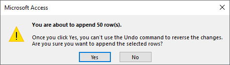
Step 10.To append the records,
Click
Step 11.To save the query, on the Quick Access toolbar,
Click , type: qappEngCourses Enter
NOTE: The "qapp" is the standard Access naming convention prefix for Append queries.
Step 12.Close the query.
Step 13.To view tblCourses,
Double-Click tblCourses
Step 14.Close tblCourses.
The one other important type of Action query is the Update query. It can be used to change data in multiple records in a table at once. This is easier than changing the records one by one.
The Faculty table holds work phone numbers for each faculty member. All of these employees currently have the area code of 812. We have just received word that some of the employee phone numbers are being assigned new area codes. Each number with a 776 exchange, as in (812) 776-2488, will switch from the 812 area code to a 444 area code.
Changing each individual phone number manually would be very time consuming. We can design an Update query to indicate which numbers need to change and modify just the area code portion of the affected numbers in one action.
Step 1.To create a new query, on the Ribbon,
Click the
Create tab, Click
Step 2.To add the table,
Double-Click tblFaculty
Step 3.Close the Show Table dialog box.
Step 4.To add the Phone field to the query design window, in the field list,
Double-Click Phone
Step 5.To select the Update Query type, on the Ribbon, in the Query Type group,
Click 
Step 6.To enter an expression to describe the numbers we will change, in the Criteria field, type:
Like "(812) 776*" Enter
NOTE: Make sure to type a space between the (812) and the 776.
Step 7.To access the Zoom tool for the Update To row, in the Phone column,
Right-Click the Update To field, Click Zoom...
Step 8.To enter an expression to describe how the phone numbers will change, type:
"(444)"+Right([Phone],9)
Step 9.To close the Zoom tool,
Click
Step 10.To preview the query result,
Click
To test the accuracy of the Update expression and its effect on the existing records, we will copy and paste the expression describing the changed numbers into a new field, change the query type back to Select query, and view the values displayed by the expression. We will see the result of the Update expression in the same way we saw the Weighted calculated field results earlier in this workshop.
Step 1.To switch to Design View,
Click
Step 2.To expand the Expr1 column,
Double-Click between the Phone column and the empty column after it
Step 3.To select the Update expression,
Press & Drag across "(444)"+Right([Phone],9)
Step 4.To copy the expression, press:
Control key+c
Step 5.To switch from an Update query to a Select query, in the Query Type group of the Ribbon,
Click 
Step 6.To create the second field, in the column to the right of the Phone field,
Click the top row, press: Control key+v, Enter
![The fields are Phone and Exp1: "(444)" + Right([Phone],9). The Phone field has a criteria of Like "(812) 776*"](/training/accam/files/pc/img/img_UpdateTestResults.png)
7.To view the query result,
Click
Step 8.Verify that yours is correct.
Now that we have confirmed the update will work as expected, we will switch the query type back to Update, and run the query.
Step 1.To switch to Design View,
Click
Step 2.To change the query type back to Update, on the Ribbon,
Click
Step 3.To run the query, on the Ribbon,
Click
Step 4.To continue with the update operation,
Click
Step 5.To close the query without saving changes,
Right-Click the
query tab, Click Close, Click
Let's check the results of the update in tblFaculty.
Step 1.To see the effect of the Update query on faculty phone numbers, in the tables list,
Double-Click tblFaculty
Step 2.To place the cursor, in the Phone column,
Click in any cell
Step 3.To sort the records by phone number, on the Ribbon, in the Sort & Filter group,
Click 
Step 4.Close tblFaculty without saving.
In spite of our best efforts to store data efficiently in databases, errors happen that result in duplication of information. Sometimes data—which may or may not be accurate—is imported from other sources. Some departments may be using databases that were poorly designed years ago, but users have continued to enter data into them anyway. And, of course, humans make data entry errors. When it is time to clean up the data, the Find Duplicates Query Wizard can help with that task.
In our database, tblStudents holds some records that have been entered over time and came from multiple sources. The possibility exists that some students may have been accidentally entered multiple times. If the primary key is entered incorrectly and doesn't match a primary key already in the table, then Access won't prevent that data from being entered. This is true of data we append from other sources or data directly entered into the database.
We will use the Find Duplicates Query Wizard to search
for duplicate records in
tblStudents.
Step 1.To activate the Create tab, on the Ribbon,
Click the Create tab
Step 2.To begin building the Find Duplicates query, in the Queries group,
Click 
Step 3.To indicate that we want to create a Find Duplicates query,
Double-Click Find Duplicates Query Wizard
Step 4.To choose the table for our search,
scroll down and Click Table: tblStudents
NOTE: We could view names for queries or for tables and queries by clicking the appropriate radio button.
Step 5.To move to the next step in the wizard,
Click 
Step 6.To select the fields with possible duplicated information,
Double-Click last_name, Double-Click first_name
Step 7.To move to the next step of the wizard,
Click
Step 8.To choose other fields for the query display,
Double-Click email, local_phone, and local_address
Step 9.To move to the next step of the wizard,
Click
Step 10.To name the query and complete the wizard, in the Name field, type:
qryStudentsFindDuplicateNames Enter
Step 11.Close the query.
The Find Unmatched Query, as its name implies, displays records in one table or query that have no match in a related table or query. For example, the Find Unmatched Query can be used to detect existing records in an inherited table that break rules of referential integrity for the database. In a sales database, for example, these might be records of orders made by a customer who does not exist in the primary customers table. When the user attempts to create a relationship and enforce referential integrity between these two tables or if he/she attempted to append new orphaned records to a table with a relationship established, Access will display an error message because of a referential integrity violation. The message states that current records in the table violate referential integrity rules, but it does not identify those records. A Find Unmatched Query will quickly discover the problem records.
We will create a Find Unmatched Query to find any sections of courses that don't have enrollments. In other words, we will check to see which sections listed in tblSections are not listed in tblEnrollments.
Step 1.To activate the Create tab, on the Ribbon, if necessary,
Click the Create tab
Step 2.To start a new query wizard,
Click
Step 3.To select and begin the wizard,
Double-Click Find Unmatched Query Wizard
Step 4.To select the table and move to the next step of the wizard,
scroll down and Double-Click Table: tblSections
Step 5.To choose the second table and move to the next step of the wizard,
Double-Click Table: tblEnrollments
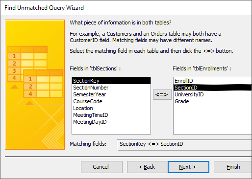
Step 6.To move to the next step of the wizard,
Click
Step 7.To choose all fields to display,
Click 
Step 8.To move to the next step of the wizard,
Click
Step 9.To name the query and finish the wizard, in the Name field, type:
qrySectionsWithoutEnrollments Enter
Step 10.Close the query.
You have seen how powerful Access queries can be in this workshop and the many varied options you have for creating and using them. Once information is gathered from data using queries, you can build forms against the query results to create a nice interface for data entry tasks, or you can build reports to share the data with others. For more information on creating forms and reports, take the Access 2016: Designing the Database Interface workshop.
We have reached the end of the workshop, so we are ready to close Access.
Step 1.Close the Access database.
NOTE: To find more training and information about Access, go to:
http://ittraining.iu.edu/Access/
We've reached the end of these materials. At IT Training, we value your opinion very much, and want to hear your feedback about what we are doing well in these materials, or how they might be improved.
If you are in our classroom, please follow your workshop instructor's guidance and take a few moments to fill out the workshop evaluation form. Also, before leaving, please log off your computer.
If you are working through these materials on your own, please take a few moments to fill out the materials' evaluation form:
http://ittraining.iu.edu/eval.aspx?mat=1730
Thank
you for participating in
Access 2016: Analyzing & Modifying
Data with Queries
Project Leader |
Jennifer L Oakes |
|
Development Team |
Mayme Fravel Donna Jones Tom Mason Kimmaree Murday Jennifer L Oakes Chris Payne |
Step 1.View the query in the query design grid.
Step 2.Open the Expression Builder.
Step 3.Create the following expression,
NOTE: Be sure to type a space between the quotes.
Step 4.Set the caption of the new field to SemesterYearSect
Step 5.Move the SemesterYearSect field after SemesterYear.
Step 6.Remove the Section Number field.
Step 7.Hide the SemesterYear field.
Step 8.To view the query result.
Step 9.Save the changes and close the query.
Step 1.Open qryCoursesSectionsAndAllFacultySummer18.
Step 2.Save it as qryCoursesSectionsAndAlFacultySemesterParameter.
Step 3.Switch to Design View.
Step 4.Change the criteria for the SemesterYear field to:
[Enter the SemesterYear] Or is Null
Step 5.Save and test the query.
Step 6.Close the query.
Step 1.Add tblCourses and tblSections to a new query.
Step 2.Change the query type to a Crosstab.
Step 3.Add the CourseTitle, and SectionNumber fields to the query
Step 4.Set the Crosstab row to Row Heading for CourseTitle and SectionNumber fields.
Step 5.To add the SemesterYear field to the query.
Step 6.Set the Crosstab row to Column Heading for the SemesterYear field
Step 7.Add the EnrollID field to the query design grid.
Step 8.Set the Crosstab row to Value for EnrollID.
Step 9.Set the Total row for the EnrollID field to Count.
Step 10.Add a EnrollID to the query design a second time.
Step 11.Set the Crosstab row to Row Heading for the second EnrollID field.
Step 12.Set the Total Field to Count for the second EnrollID field.
Step 13.Set the caption for the second EnrollID field to Total Enrollments.
Step 14.View the query.
Step 15.Save the query and close it.
