Whether we want to put our data in a different order (alphabetical, sequential, etc.) or see only specific parts of the data, Google Sheets has features that make sorting and filtering data quick and easy.
Copying the practice workbook
If you are beginning this course at this point, you will need to copy the practice workbook to your Google Drive.
- To begin copying the practice workbook in a new browser window,
Right-Click Copy practice workbook, Click Open link in new window
The file begins to open in a new window of the web browser. Before the document will open and can be edited, we need to make a copy of it.
Move to the new browser window.
- To copy the workbook file, in the browser window,
Click ![]()
A copy of the file is now open and, by default, is saved in your Google Drive. The filename now has the words "Copy of" at the beginning.
Sorting data
Currently, the data in the Sales by Location worksheet is in alphabetical order by location. Let's change this to be organized in ascending order by date.
Before sorting data in Google Sheets, it is important to freeze the header row. This will keep the first row of the worksheet, which contains the column headers, from being sorted with the data.
- To select the header row, on the left side of the worksheet,
Click

- To freeze the header row, on the menu bar,
Click View, Point Freeze, Click 1 row
- Deselect the header row.
- To see options for the Date column,
Point
 , Click
- To sort by date, in the drop-down menu,
Click Sort sheet A to Z
- To deselect column A,
Click in a blank cell
The data is now in ascending order with the oldest date (6/5/2022) at the top.
Filtering data
Google Sheets also gives us an easy way to filter data. When data is filtered, it is hidden but not removed, so no data is lost.
Let's filter the data to see just the sales that will benefit the food pantry.
- To create a filter, in the menu bar,
Click Data, Click Create a filter
All of the data is selected. The column headings have small icons to the right of their names.
![]()
These icons can be used to open filtering, and sorting, options.
- To open the filtering options, in the Beneficiary column,
Click

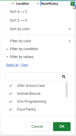
The Beneficiary sort and filter drop-down menu opens:

The drop-down menu has the sorting options at the top. The filtering options are at the bottom of the menu. Each unique value, in this case, Beneficiary, is listed. Removing the checkmark next to a value hides that value.
We want to remove all of the beneficiaries except the Food Pantry. We could uncheck each beneficiary. Or we can clear all of the checkmarks and then check just the Food Pantry entry.
- To deselect all of the beneficiaries, in the middle of the drop-down menu,
Click Clear
- To select just the Food Pantry,
Click Food Pantry
- To accept this filter,
Click

The data has been filtered and only shows the dates and locations when the Food Pantry was the beneficiary.

Notice the row numbers. Only the rows containing the Food Pantry are visible. The other rows are hidden. In addition, the icon next to the column header has changed and now looks like a small filter. This tells anyone who looks at this worksheet that the data is filtered by this column.
- To open the Beneficiary filtering options,
Click

- To remove the filter, in the middle of the drop-down menu,
Click Select all
- To accept this change,
Click

If you have been working through this course in sequential order, you have reached the end of the materials.

