When data is entered into a spreadsheet, by default, the General format is applied. The General format left aligns text and right aligns numbers. There are other types of formats that can be applied, including but not limited to Number, Currency, and Date. Occasionally there is data that doesn't fit one of the predefined formats. In these cases, we can use a Special format or even create a Custom format.
Copying the practice workbook
If you are beginning this course at this point, you will need to copy the practice workbook to your Google Drive.
- To begin copying the practice workbook in a new browser window,
Right-Click Copy practice workbook, Click Open link in new window
The file begins to open in a new window of the web browser. Before the document will open and can be edited, we need to make a copy of it.
Move to the new browser window.
- To copy the workbook file, in the browser window,
Click ![]()
A copy of the file is now open and, by default, is saved in your Google Drive. The filename now has the words "Copy of" at the beginning.
Creating custom cell formats
If there isn't a predefined cell format for the data, a Custom format can be created and applied. Custom formats can be used for many types of formatting including standard text, decimal point alignment, leading zeros, and date formatting.
With the address information separated into four columns, it may be more evident that the zip codes aren't quite right. Some of them are only four digits. A standard United States zip code uses five numbers. In many parts of the eastern U.S., the zip codes start with a zero (0). When the address data was separated and the zip codes were moved to column K, Google Sheets treated them as numbers. Sheets doesn't allow numbers to start with zero (0) and automatically removed that digit. Although zip codes are technically numbers, they aren't used in mathematical functions and are treated as text.
Let's create a custom format that will require the cells containing the zip codes to have five digits.
- To select column K, in the header row,
Click the column K header
- To open the Custom number formats dialog box, on the menu bar,
Click Format, Point Number, Click Custom number format
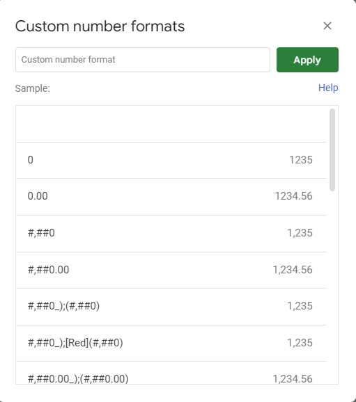
The Custom number formats dialog box appears:
We want to require the cells that contain the zip codes to have five digits. To do this, we will enter five zeros into the Custom number format field.
- To correctly place the cursor,
Click in the Custom number format field
- To create a five-digit custom format, type:
00000, Click

- Deselect the cells.
The leading zeros have been returned to the appropriate zip codes.
The Employee ID numbers in column A are all five digits. Let's update this so that there is a hyphen between the second and third digits. We will create a Custom cell format and apply it to all of column A. When finished, the ID numbers will look like this: 34-567.
- To select column A, in the header row,
Click the column A header
- To open the Custom number formats dialog box, on the menu bar,
Click Format, Point Number, Click Custom number format
To create this custom format, we will use zeros as placeholders for numbers and will add the hyphen between the second and third digits. The format will look like this: 00-000.
- To correctly place the cursor,
Click in the Custom number format field
- To create a five-digit custom format, type:
00-000, Click

- Deselect the cells.
The Employee ID numbers are now formatted with a hyphen between the second and third digits. Because the formatting was applied to the entire column, if a new employee is added, the ID number will automatically be formatted that way. The person inputting the information will not have to type the hyphen.

