This fictional credit card data can give us a lot of information about our spending habits. Because the balance isn't paid off each month, the individual statements (January, February, and March) are connected. We can use information from one month to help analyze data in other months.
Copying the practice workbook
If you are beginning this course at this point, there are two practice workbooks you will need to copy to your Google Drive.
- To begin copying the first practice workbook, Copy of Google Sheets: Working with non-numeric data: Working across worksheets, in a new browser window,
Right-Click Copy practice workbook, Click Open link in new window
The file begins to open in a new window of the web browser. Before the document will open and can be edited, we need to make a copy of it.
Move to the new browser window.
- To copy the workbook file, in the browser window,
Click ![]()
A copy of the file is now open and, by default, is saved in your Google Drive. The filename now has the words "Copy of" at the beginning.
- To begin copying the first practice workbook, Monthly_Statements, in a new browser window,
Right-Click Copy practice workbook, Click Open link in new window
The file begins to open in a new window of the web browser. Before the document will open and can be edited, we need to make a copy of it.
Move to the new browser window.
- To copy the workbook file, in the browser window,
Click ![]()
A copy of the file is now open and, by default, is saved in your Google Drive. The filename now has the words "Copy of" at the beginning.
Copying a worksheet
NOTE: If you are continuing from the previous section, your files will be named, Copy of MarchStatement and Copy of Google Sheets: Working with non-numeric data: Working with external data. If you are beginning in this section, your file will be named, Copy of MarchStatement and Copy of Google Sheets: Working with non-numeric data: Working across worksheets.
Currently, our fictional credit card statements are in two different workbooks, Copy of MarchStatement and Copy of Google Sheets: Working with non-numeric data: Working across worksheets. Before we begin analyzing the data, let's copy the March_Statement worksheet into the Copy of Google Sheets: Working with non-numeric data: Working across worksheets workbook.
When the worksheet is copied, Google Sheets will automatically open a new copy of the Copy of Google Sheets: Working with non-numeric data: Working across worksheets workbook. To avoid confusion, let's close the workbook before we start the process of copying the worksheet.
- To close the Copy of Google Sheets: Working with non-numeric data: Working across worksheets workbook, if necessary, in the browser,
Close the Copy of Google Sheets: Working with non-numeric data: Working across worksheets tab
- To open the "Select a spreadsheet to copy this worksheet into" dialog box, at the bottom of the workbook,
Right-Click the March_Statement tab, Point Copy to, Click Existing spreadsheet
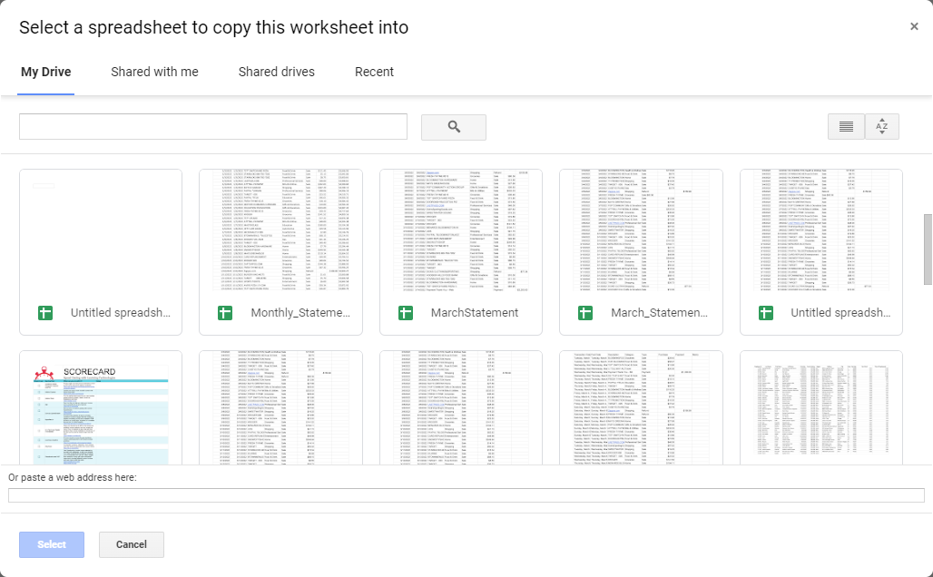
The "Select a spreadsheet to copy this worksheet into" dialog box opens:

This dialog box prompts you to select a spreadsheet from My Drive, Shared with me, Shared drives, or Recent files. The Copy of Google Sheets: Working with non-numeric data: Working across worksheets spreadsheet was copied into My Drive. Depending upon the structure of your Google My Drive, you may see folders and files.
- To select the Copy of Google Sheets: Working with non-numeric data: Working across worksheets spreadsheet, in the "Select a spreadsheet to copy this worksheet into" dialog box,
Double-Click

A notification that the sheet was successfully copied appears.
- To open the Copy of Google Sheets: Working with non-numeric data: Working across worksheets spreadsheet, in the notification,
Click Open spreadsheet
The Copy of Google Sheets: Working with non-numeric data: Working across worksheets workbook opens. It now contains four worksheets, January, February, Spending, and Copy of March_Statement.
Rearranging worksheets
The Copy of March_Statement worksheet was placed at the end of the row of worksheet tabs. However, it would make sense for this to go after the February worksheet tab.
We could use the Move or Copy dialog box to place this worksheet where we want it. But let's try a different method. We'll Press & drag the worksheet tab to the correct location.
- To move the Copy of March_Statement worksheet,
Press & drag the Copy of March_Statement worksheet tab to the left until the tab is between the February and Spending tabs
The worksheet tabs are now in the correct order:
![]()
Before we move on, let's rename the Copy of March_Statement worksheet so that it better matches the other months.
- To select the current name,
Double-Click the Copy of March_Statement worksheet tab
- To rename the worksheet, type:
March Enter key
Referencing cells in another worksheet
The January and February worksheets both have a Balance column. This column calculates the balance as charges and payments are made. The beginning balance of each month is the ending balance of the previous month. Let's add a Balance column to the March worksheet and use February's ending balance as a starting point.
- Move to the March worksheet, if necessary.
- To add the Balance heading,
Click in cell H1, type: Balance
With the Balance heading in place, we are ready to reference a cell in the February worksheet as the previous balance.
- Make cell H2 the active cell, if necessary.
- To begin referencing the cell, type:
=
- To move to the February worksheet, at the bottom of the workbook,
Click the February tab
- To reference the correct cell, in the February worksheet,
Click cell H109
- To accept H109 as the correct cell and return to the March worksheet, on the keyboard, press:
Enter key
The February balance, 1836.05, appears in cell H2.
Let's take a moment to look at the formula in cell H2.
- To return to cell H2, if necessary, on the keyboard, press:
Up Arrow key
The formula in cell H2 is:
=February!H109
The name of the worksheet being referenced, February, is followed by an exclamation point. The data after the exclamation point is the cell reference.
With the previous balance in place, we can now create a formula that will calculate the balance with each purchase and payment. To do this, we will use the closest balance amount which will be in the row above the selected cell. We will put this formula in cell H3 and copy it down the rest of the column.
- Make cell H3 the active cell.
- To begin the formula and reference the closest occurrence of the balance, type:
=h2
- To add purchases to the formula, type:
+f3
- To add the negative payments, type:
+g3
The formula looks like this: =h2+f3+g3
- To accept the formula, press:
Enter key
Because some of the cells in column G are blank, Double-Clicking the auto-fill handle to copy the formula down column H will not work. We will use another method.
- To return to cell H3, on the keyboard, press:
Up Arrow key
- To copy the formula,
Right-Click cell H3, Click Copy
- To select the rest of column H,
Press & Drag H4:H114
- To paste the formula into the selected cells,
Right-Click the selected cells, Click Paste
- To widen column H, in the header row,
Double-Click between column H and column I
- Deselect column H.
Referencing an entire column
The workbook contains a fourth worksheet named Spending. In this worksheet, we track the spending for each month. The spending is calculated by adding up all of the purchases for the month. This could be done by using the SUM function and referencing all of the cells that contain a purchase. For example: =SUM(March!F3:F115). However, each month will have a different number of purchases and different cell references. In addition, typing or selecting the cells leaves room for error. To simplify this, we can reference an entire column.
Referencing an entire column is done by typing the column letter, a colon, and the column letter a second time. For example, =SUM(March!F:F). This function will add together all of the values contained in column F.
Let's move to the Spending worksheet and add the March spending total.
- To move to the Spending worksheet, at the bottom of the workbook,
Click the Spending tab
- To see the function in cell B2,
Click in cell B2
The function to calculate the January spending is =SUM(January!F:F).
- Make cell B3 the active cell.
- To begin entering the SUM function, type:
=sum(
- To enter the worksheet reference, type:
March!
- To enter the reference to the entire column, type:
F:F)
- To enter the function, on the keyboard, press:
Enter key
The total spending for March, $4,855.98, appears in cell B3.
- To return to the March worksheet, at the bottom of the browser window,
Click the March worksheet tab

