Let's create a pivot table, based on the AlumniDonors worksheet, that will show us information about donations (number, total, and average) based on donation date and campus. To see three different types of data, there will need to be multiple fields in the Values area of the Pivot table builder.
Copying the practice workbook
If you are beginning this course at this point, you will need to copy the practice workbook to your Google Drive.
- To begin copying the practice workbook in a new browser window,
Right-Click Copy practice workbook, Click Open link in new window
The file begins to open in a new window of the web browser. Before the document will open and can be edited, we need to make a copy of it.
Move to the new browser window.
- To copy the workbook file, in the browser window,
Click ![]()
A copy of the file is now open and, by default, is saved in your Google Drive. The filename now has the words "Copy of" at the beginning.
We want to see three types of information about the donation amounts: the total number, total amount, and average amount. To accomplish this, we will add the Donation Amount field to the pivot table Values area three times. By default, Google Sheets will sum the donation amounts and provide the total amount of donations. We will use the Value Field Settings dialog box to change the calculation for the other two occurrences of the field to show the total number and average amount.
- Move to the AlumniDonors worksheet, if necessary.
- To begin creating the pivot table, on the menu bar
Click Insert, Click Pivot table
- To accept the range and placement and place the pivot table in a new worksheet, in the Create pivot table dialog box,
Click

- To name the pivot table worksheet,
Double-Click the new worksheet tab, type: DonationsByDate Enter key
- To add the Donation Amount field to the Values area,
Press & Drag the Donation Amount field to the Values area
- Add the Donation Amount field to the Values area two more times.
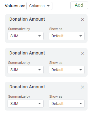
The Donation Amount field is now in the Values area three times:

Each occurrence is summarized by the SUM function. We can change this to see different functions applied to the Donation Amount.
- To change the Summarize by option to Count, in the first Donation Amount field,
Click
 , Click COUNT
With the first Donation Amount field now showing the number of donations, we will use the same process to change the second field to show the average amount.
- To change the Summarize by option to Count, in the second Donation Amount field,
Click
 , Click AVERAGE
With the three value fields set up, let's take a moment to format them and make them easier to understand. We'll change the names of the fields and widen the columns to fit the text.
- To change the name of the Count of Donation Amount field,
Click cell A1, type: Number of Donations
- To change the name of the Average of Donation Amount2 field,
Click cell B1, type: Average Donation
- To change the name of the Sum of Donation Amount3 field,
Click cell C1, type: Total Donations
- To select the columns, in the column header,
Press & Drag column A to column C
- To widen the columns, in the column headers,
Double-Click

- To deselect the columns,
Click in the pivot table
With the value fields formatted correctly, we can add the remaining fields to the pivot table. We want to analyze the donation data based on donation date and campus. We will add both of these fields to the Rows area.
Grouping by date in a pivot table
When working with Google Sheets, we can use a date field multiple times to see different date groupings such as year, month, quarter, day, etc. We want to see the donations by year, month, and date. We will add the Donation Date field to the Rows area three times. This works differently than the previous exercise with the Donation Amounts. When working with the dates, it is necessary to adjust each occurrence before adding the next one.
- To add the Donation Date field to the Rows area,
Press & Drag the Donation Date field to the Rows area
By default, the Donation Date data comes in as individual dates. Let's group these dates by year.
- To see the pivot date group options,
Right-Click cell A2, Point to Create pivot date group
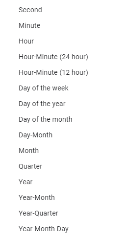
The pivot date group options open:

The pivot date options range from second to year. Our data is not detailed enough to group by the second, minute, or hour. We want to see our data by year, month, and day.
- To group by year, month, and day, in the pivot date group options,
Click Year-Month-Day
The dates in the pivot table change slightly. They are now in a year-month-day format. Each date that has a donation is listed. Some dates have only one donation. Some dates have multiple donations.
This isn't exactly what we wanted. We want to see the donations by year and then months within each year. Let's remove this grouping and try again.
- To remove the current grouping,
Right-Click a cell that contains a date, Click Ungroup pivot items
The dates are returned to their original format. Now let's group them by year.
- To group the dates by year,
Right-Click a cell that contains a date, Point Create pivot date group, Click Year
We now see the donation data by year.

While this is helpful, we also want to see the donation information by month. To accomplish this, we will need to add the Donation Date field to the Rows area a second time.
- To add the Donation Date field to the Rows area,
Press & drag the Donation Date field to the Rows area under Donation Date - Year
The pivot table adjusts, and columns are shifted to the right. The years in column A have expanded and the individual dates are visible in column B.

We will modify the second occurrence of the Donation Date field to be grouped by months.
- To group the dates by month,
Right-Click a cell in column B that contains a date, Point Create pivot date group, Click Month
Column B now shows each month of each year. The annual totals are at the end of each year.
Let's add the Donation Date field to the pivot table one last time so that we can see the individual dates within each month.
- To add the Donation Date field to the Rows area,
Press & drag the Donation Date field to the Rows area under Donation Date - Month
The pivot table now shows the donation information by year, month, and day.

The months and years in the pivot table can be collapsed and expanded to see more or less information.
- To collapse the Donation Date - Year field, in the pivot table,
Right-Click cell A2, Click Collapse all in Donation Date -Year
- To expand the 2018 Total field,
Click

The pivot table now shows us the annual totals for 2016, 2017, 2019, and 2020. As well as the monthly and daily totals for 2018.
- To collapse the 2018 field, in the pivot table,
Click


