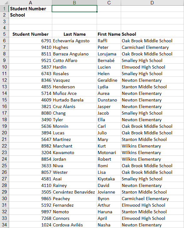
VLOOKUP is a function in Microsoft Excel and Google Sheets that looks for specific data in a range of cells and then returns corresponding data. For example, as demonstrated in this sample worksheet that contains student information, we could use the VLOOKUP function to return the school when the student number is entered.

We will become familiar with the VLOOKUP syntax and then move on to entering VLOOKUP functions.
NOTE: This course will cover the VLOOKUP function in both Microsoft Excel and Google Sheets. While the VLOOKUP function works the same in both programs, there are slight variations in the interface and terminology. These differences will be described where necessary throughout the course.
Understanding the VLOOKUP function
The VLOOKUP function looks for a value (text or numeric) in the first column of a set of data and then returns a related value from a specified column in the data.
Microsoft Excel and Google Sheets have different syntax for the arguments used in the VLOOKUP function.
Microsoft Excel VLOOKUP function: =VLOOKUP(lookup_value, table_array, col_index_num, range_lookup)
Google Sheets VLOOKUP function: =VLOOKUP(search_key, range, index, [is_sorted])
While the syntax of these functions looks very different, they work in exactly the same way.
The VLOOKUP arguments are described here:
- lookup_value/search_key: The actual value or cell reference you are looking up. This value can be within the range or on a different worksheet or workbook.
- table_array/range: The range of cells that contains the lookup values. It is recommended that this be a named range. The first column of this range must contain the values you are looking up.
- col_index_num/index: The column number from where a value should be returned. This does not necessarily correspond to the column header.
- range_lookup/[is_sorted]: This argument specifies whether you want to return an exact match or an approximate match. There are two possible values: FALSE or TRUE. Do you want an exact match? If so, enter FALSE. Do you need an approximate match? Enter TRUE. (While the FALSE and TRUE designations may seem counterintuitive, remember that FALSE and "exact" both have five letters.)
In other words, the argument is composed of the following pieces of information: =VLOOKUP(the value you are looking for, where you are looking for the value, the value you want to be returned, exact or approximate match).
To examine this further, let's look at the VLOOKUP function used in the following example: =VLOOKUP(B1, A5:B34, 4, false).
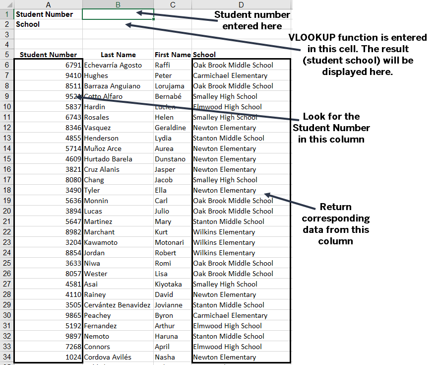
This VLOOKUP function is intended to return the student's school when the Student Number is entered and is placed in the cell where we want the result, cell B2. This function is telling the spreadsheet to look for the value in cell B1 in the range A5:B34, when the value is found in the first column of the range, return the value from the fourth column of the same row. The value in the first column should be an exact match to the value in cell B1. This is illustrated in the following image:

Let's open a file and work with the VLOOKUP function.


