In the previous sections, we saw how to use the false argument in the VLOOKUP function to return an exact match. There may be times when an approximate, or closest, match is desired. For example, a grading scale or a range of dates. In these spreadsheets, we want the VLOOKUP function to find the closest value without going over. When looking for an approximate match, the range where you are searching must be organized in ascending order.
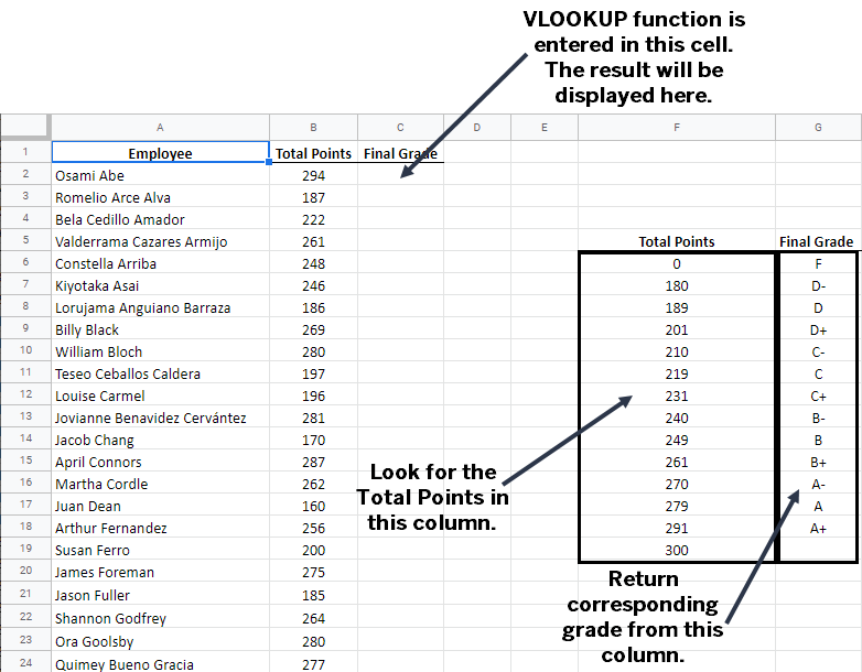
In the following example, we are looking for a student's final grade. Grade assignments typically span several points. A student's total points may not exactly match the points listed. By using the true argument within the VLOOKUP function, we can find the closest total points.
=VLOOKUP(B2,$F$6:$G$19,2,true).
This function is saying, "Look for the value in cell B2 in the first column of the range F6:G19. When a value higher than the value of cell B2 is reached, stop and go back to the previous value, and return the final grade in the 2nd column." The following image shows this in more detail.

NOTE: This VLOOKUP example uses absolute cell references. These references are discussed in the section titled Using absolute cell references in the VLOOKUP function.

