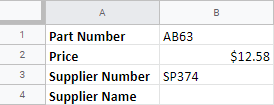
More than one VLOOKUP function can be used in a worksheet. Let's add a second one to return the supplier number in addition to the price when we search for the part number.
Acquiring the practice workbook
If you are beginning this course at this point, you will need to access the practice workbook.
Downloading the practice workbook for Microsoft Excel
If working in Microsoft Excel, you will download and extract the workbook.
- To begin downloading the practice workbook, click the following button:
For detailed instructions on downloading and extracting files in Google Chrome or Firefox, visit Getting Started with Exercise Files.
Copying the practice workbook in Google Sheets
In Google Sheets, you will copy the workbook to your Google Drive.
- To begin copying the practice workbook in a new browser window,
Right-click Copy practice workbook, Click Open link in new window
The file begins to open in a new window of the web browser. Before the document will open and can be edited, we need to make a copy of it.
Move to the new browser window.
- To copy the workbook file, in the browser window,
Click ![]()
A copy of the file is now open and, by default, is saved in your Google Drive. The filename now has the words "Copy of" at the beginning.
Adding a second VLOOKUP function
We are still working in the Bike Parts worksheet. We need to adjust the worksheet so that when a user searches for a part number, not only is the price returned, but the supplier number is as well. This can be accomplished by adding a second VLOOKUP function to cell B3, Supplier Number.
Let's move to the correct cell and start entering the function. Remember, the first argument of the function tells the spreadsheet what we are looking for.
- To make cell B3 the active cell,
Click in cell B3
- To begin entering the function, type:
=vlookup
- To enter the first argument, type:
(b1,
The second argument in the VLOOKUP function tells the spreadsheet where to look for the value in cell B1 (part number). In this case, we want to look in the parts list, A7:D16.
- To add the range to the function, type:
a7:d16,
The third argument tells the spreadsheet which column contains the data you want to be returned. We want the supplier number to be returned. The supplier numbers are in the second column of the range. Therefore, we will add "2" to the function.
- To add the column number, type:
2,
The final argument tells the spreadsheet if you want an exact match (false) or an approximate match (true). We are looking for an exact part number, so we will use the false argument.
- To specify an exact match, type:
false)
The function should look like this: =VLOOKUP(b1,a7:d16,2,false).
- To enter the function, on the keyboard, press:
Enter key
The supplier number associated with part number AB222, SP363, appears in cell B3.
NOTE: Depending on the part number entered in cell B1, the supplier number displayed might be different.
Let's change the part number and see both VLOOKUP functions in action.
- To enter a different part number,
Click in cell B1, type: AB63 Enter key
Both the price and supplier name fields adjust to reflect part AB63.

Now let's see how to create a VLOOKUP function using values on another worksheet.

