Grouping Worksheets

Grouping worksheets allows a number of tasks to be performed similarly on all sheets in a group at the same time. For example, you could enter text in the same cell, name headers and/or footers, run spell check, or send to the printer for all grouped sheets at once.

Let's group the worksheets together so that we can quickly label all of the columns and rows and streamline the organization of data. Then, we will add data to the worksheets and explore a couple of ways to easily summarize the data across these sheets.

Step1. To select the worksheets to group,

Click the Jan tab, hold Shift key+Click the Mar tab

All of the selected tabs take on a white background and the word [Group] appears in the window's title bar, after the filename. This is the indicator that multiple worksheets have been selected, and will be treated as a group.

Let's see how to do this. We'll enter the row labels first, then the column labels.

Step1. To enter the row labels starting in cell A1, type:

Item Enter Coffee Enter Tea Enter

Step2. To enter the column labels,

Click cell B1, type: Morning Tab key Afternoon Tab key Evening Enter

The row and columns labels are entered, and the active cell is now cell B2. Now we will do some light data entry, but we will do it without all of the sheets grouped together. Let's look at the contents of the other sheets first.

Step3. To move to the Feb worksheet,

Click the Feb worksheet tab

You see the same row and column labels occupying the same range. Let's add some data to this sheet.

Step4. To enter the data for this worksheet, type:

10 Tab key 20 Tab key 30 Enter,
5 Tab key 10 Tab key 15 Enter

The data is entered on the Feb worksheet. It now looks like this:

Now we'll do something similar on the Mar worksheet.

Step5. To move to the Mar worksheet,

Click the Mar worksheet tab

You see the same row and column labels occupying the same range as on the other two worksheets. Let's add some data to this sheet, too.

Step6. To enter the data for this worksheet, type:

20 Tab key 30 Tab key 40 Enter,
10 Tab key 15 Tab key 20 Enter

The data is entered on the Mar worksheet. It now looks like this:

Now we'll add some data back on the Jan worksheet.

Step7. To return to the Jan worksheet,

Click the Jan worksheet tab

Step8. To enter the data for this worksheet, type:

1 Tab key 2 Tab key 3 Enter,
1 Tab key 2 Tab key 3 Enter

The data is entered on the Jan worksheet. It now looks like this:

Step9. Save the workbook, Grouped.xlsx.

Now we have three worksheets containing data. The worksheets all have the same structure (similar labels and data in the same locations on each sheet). Now we will explore a couple of ways to summarize the data, across all of the worksheets. The first will use the Consolidate feature, and the other will use a 3-D formula to reference multiple worksheets at once.

Summarizing Data Across Worksheets

There are actually three different ways to summarize data across multiple worksheets, which could exist in multiple workbooks. Today, we'll look at a simpler example, where all of them are in the same workbook. All three possible ways still apply. The ways to summarize across multiple worksheets depend on what you are trying to do with the data, how the data is structured and organized, and whether you want the data to remain dynamic or if a snapshot of it is sufficient for your needs. The three ways to summarize data across worksheets are:

• Consolidate by category: when the row and column labels are the same, the items or number of items may be different from within the data sources, and you want to use some kind of summarizing function on the data (e.g., SUM, COUNT, AVERAGE,...).
• Consolidate by position: the data is very highly structured; row and column labels match exactly by wording and position, and the data within them is arranged in the same order and position. Use this if the data sources all used the same template, and you want to use some kind of summarizing function on the data (e.g., SUM, COUNT, AVERAGE,...). There should be no blank rows or columns in your data.
• Use a formula: the most flexible method, but requires the most effort.

Which method you use will depend on your own data and needs. Let's add a worksheet to this workbook, and use the consolidate by position option in that new worksheet.

Step1. To create a new worksheet in the workbook,

Click

Step2. To begin to change the worksheet name,

Double-Click the Sheet# worksheet tab name

Step3. To rename the worksheet, type:

Cons Enter

The worksheet is now named Cons. Let's move it to the end of the row of worksheet tabs.

Step4. To reposition the Cons worksheet to the end,

Press & Drag the Cons worksheet tab to the right of the Mar worksheet tab

Let's place the active cell in the upper left corner, if it isn't already there.

Step5. To move the active cell, if necessary,

Click cell A1

This active cell is where our consolidated data will begin.

Now that our worksheet is prepared, let's explore the consolidate by position capability for summarizing data.

Consolidating Data by Position

By grouping the worksheets to create their structure, the result is similar to if we had used a template: the data is all in the same order and position across the worksheets, and the row and column labels all match exactly. This means we can use consolidate by position to obtain a summary of all the data in the first three worksheets.

Let's see how to do this.

Step1. Switch to the Data command tab.

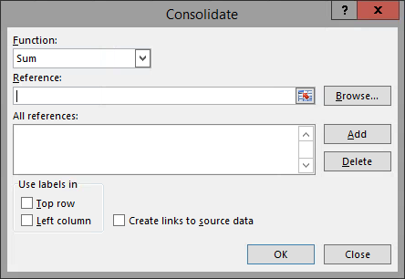
Step2. To begin to consolidate the data, in the Data Tools group,

Click

You see the Consolidate dialog box appear:

NOTE for MacOS Users: The appearance of the contents of the Consolidate dialog box is slightly different, but the functionality is the same.

In the Function field, we are able to change which summary function we want to use to consolidate the data. By default, it uses the Sum function. We'll leave that setting as it is.

Now we will need to specify the ranges where our data exists.

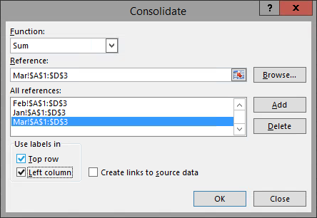
Step3. To begin to specify the first desired data range, in the Reference field,

Click

The dialog box collapses to just the References field.

Step4. To select the desired data range,

Click the Jan tab, Press & Drag the range A1:D3, Click

You see the range "Jan!$A$1:$D$3" appear in the Reference field.

NOTE for MacOS Users: To make the selected range appear in the "All references:" field, Click.

Step5. To confirm this range as a data selection,

Click

The range Jan!$A$1:$D$3 appears in the All References field.

Step6. Repeat steps 3-5 to add the ranges for the Feb and Mar worksheets.

Now we will specify the labels to be used.

Step7. To specify the location of the desired labels in the selected references, near the bottom of the dialog box,

Click the Top row checkbox, Click the Left column checkbox

Both checkboxes are toggled on. Now we can specify how the consolidation should be updated. If we leave the "Create links to source data" checkbox unchecked, we will have to manually update the reference ranges if their data should change. If it is checked, any changes would be automatically seen in the consolidated data summary.

Let's leave it unchecked for right now, and we will update it manually later.

The Consolidate dialog box should look similar to this:

8. To confirm all of these changes,

Click

The consolidated summary appears in the Cons worksheet. It now looks like this:

Notice that the Consolidate feature dropped the first label (Item) in the range.

Step9. Save the workbook, Grouped.xlsx.

Consolidating Data with a 3-D Formula

We can analyze data in the same cell (or range) on multiple worksheets within a workbook by using a 3-D reference in a formula. The syntax for a 3-D reference begins with the range of worksheet names, followed by the cell or range reference. If we had a workbook with four worksheets named Sheet1, Sheet2, Sheet3, and Sheet4, and we wished to add up the contents of the cells B3 on just the last three sheets, we would use the formula =SUM(Sheet2:Sheet4!B3). A 3-D formula can be used with many common functions, including SUM, AVERAGE, COUNT, MAX, MIN, and others.

Let's use a 3D formula to confirm the result of the Consolidate feature. First, we'll use a formula to replicate the row and column labels. We'll start our formula in cell B5.

Step1. Move the active cell to cell B5.

Step2. To create a formula linking cell B5 to the contents of cell B1, type:

=B1 Enter

Step3. Copy the formula in cell B5, and paste it into the range B5:D5.

Step4. Copy the formula in cell B5, and paste it into the range A6:A7.

Now the new range has the same row and column labels as the consolidated range above. This pasting works because we are maintaining the relative references between the cells' locations.

Now we will create a 3D formula to gather the data across the target worksheets.

Step5. To create a 3D formula in cell B6, type:

=sum(Jan:Mar!B2 Enter

Excel completes the formula, adding the "missing" right parenthesis. The formula result, 31, appears in cell B6.

Step6. Copy the 3D formula in cell B6, and paste it into the range B6:D7.

The values displayed in each tabular section should match the other right now.

Now let's see what happens if the source data changes. We will change the value in cell B2 of the Feb worksheet to be 50.

Step7. Switch to the Feb worksheet.

Step8. To change the value in cell B2,

Click cell B2, type: 50 Enter

The contents of cell B2 change to 50. Now let's see what happened in the two summary ranges we created on the Cons worksheet.

Step9. Switch to the Cons worksheet.

The range with the 3D formula has updated to show the changed data. The range created with the Consolidate feature is not changed, because it was created without checking the "Create links to source data" checkbox, and so requires manual updating of the source data changes.

Updating Consolidated Data Manually

When consolidating data by position, you can choose to have the summarized data range update automatically. If you do not specify that initially and the reference data changes, you can still update the summarized data manually.

Let's see how to do this.

Step1. To select the range and labels using the consolidate feature, on the Cons worksheet,

Press & Drag the range A1:D3

Step2. To begin to manually update the consolidated range, on the Data tab, in the Data Tools group,

Click

You see the Consolidate dialog box.

Step3. To update the data in the references,

Click

The summarized data range updates, and now matches the range created with the 3D formula.

NOTE: Performing this process for manually updating the consolidated range may also be used to change the status of the "Create links to source data" checkbox, if desired.

Step4. Save the workbook, Grouped.xlsx.

Grouping worksheets can also be used for other tasks, such as quickly creating consistent headers or footers across multiple worksheets. Let's see how to do that.

Grouping for Consistent Headers or Footers

In addition to creating a consistent structure on multiple worksheets at the same time, grouping worksheets allows you the ability to quickly create custom headers or footers across the entire group of worksheets.

Since we began today with a new workbook, it does not have anything in the header. Let's group the worksheets together, and create the same custom header on all of them at once.

Step1. To select the worksheets to group, on the tabs at the bottom of the workbook,

Click the Jan tab, hold Shift key+Click the Cons tab

NOTE: If you have several worksheets, the Control key or the Command key can be used to select multiple individual worksheets to be grouped.

All of the selected tabs take on a white background and the word [Group] appears at the top of the window after the file name.

Step2. To view the headers in Print Preview, on the Ribbon,

Click the File tab, Click Print

NOTE for MacOS Users: To view the headers in Print Preview, on the Menu bar, Click File, Click Print...

You see the Jan worksheet in Print Preview mode. At the center bottom of the window you see a navigation tool for moving from page to page. Because the worksheets are grouped, all of the grouped sheets are being treated as one print job. So even though the Jan worksheet would be just one page, this view includes all the pages it would take to print all of the selected worksheets.

Step3. To preview a different worksheet, below the print preview,

Click

NOTE: Your total number of pages may vary.

So we see two advantages of grouping worksheets in this example: the ability to perform the same action on many worksheets at once and to print all of them at once. Let's see how to add a header to all sheets in this workbook at once by grouping them.

Step4. To exit the Print Preview and leave the Backstage view,

Click

NOTE for MacOS Users: To exit the Print dialog, Click Cancel.

Step5. Verify the worksheets are still grouped, and group them, if necessary.

Step6. To access the worksheets' headers,

Click the Insert tab, Click

You see three sections of the worksheet header - left, middle and right. We'll put the current date and time (according to the computer Excel is running on) in the left section in a way that it will update automatically each time we work with the file. Then any printing will always have a current date/time stamp in the header.

Step7. To add the current date to the header,

Click in the left section, Click

You see a placeholder (&[Date]), which will be interpreted to display the current date whenever this file is opened. Now let's add the current time to this section as well.

Step8. To add the current time to the header, press:

Spacebar, then Click

The section now displays more code (&[Date] &[Time]). This will cause Excel to update this placeholder to the current date and time when the worksheet is printed.

Now let's add the worksheet name to the right side of the header.

Step9. To add the worksheet name to the right section of the Header,

Click in the right section, Click

You see the code &[Tab] which, for each worksheet, will be replaced with the name of the worksheet tab.

NOTE for MacOS Users: To continue, you must move the active selection from the Header area, Click anywhere in the data area of the worksheet.

Step10. To preview the headers, on the Ribbon,

Click the File tab, Click Print

NOTE for MacOS Users: To view the headers in Print Preview, on the Menu bar, Click File, Click Print...

The header is displayed with the current date on the left and the worksheet name at the right:

Next we will ungroup these worksheets, since we are finished working with them as a group.

Step11. To exit the Print Preview and leave the Backstage view,

Click

NOTE for MacOS Users: To exit the Print dialog, Click Cancel.

Step12. To return to regular view of the workbook, on the Ribbon,

Click the View tab, Click Normal

To ungroup worksheets, we can select any one worksheet tab.

Step13. To ungroup the worksheets,

Click any worksheet tab

The tab colors should display again, and the [Group] indicator should no longer appear in the title bar of the Excel window.

Step14. Save the workbook, Grouped.xlsx.

NOTE: Another way to accomplish what we have done by grouping worksheets is by using a macro. For more information on creating and working with macros, consider attending the IT Training workshop Excel 2016: Basic Automation Using Macros.