Importing and Cleaning Data

External data is data that is stored outside of Excel. Excel easily works with data created in different applications if this data is saved in a format Excel can recognize. We may want to import data from another database that meets certain criteria. By importing the data into Excel, we can still manipulate and format the data using the tools in Excel.

Often, when using Excel, you will be getting your data from another source, and it will need to be cleaned up before you can begin analyzing it. The Microsoft Support site has a long list of recommendations for cleaning up data.

The core steps for cleaning data are:

1. Import the data from the external data source.
2. Make a backup copy of the unmodified imported data in a separate workbook.
3. Make sure the data conforms to a tabular format of rows and columns with:
   • similar data in each column.
   • all columns and rows visible.
   • no blank rows or columns within the range.
4. Next, do any tasks that don't require manipulation of all of the data in an entire column first (e.g., spell-checking or using Find and Replace).
5. Finally, do the tasks that require manipulation of all of the data in an entire column.

Having the backup of the imported data provides a safety net to perform the other, potentially more destructive (intentionally or not) tasks.

Let's see how some of these core steps might actually be performed now.

Spoiling the Game of Thrones Book Series

For this next section, we have a text file containing data about characters from the book series, A Song of Ice and Fire, and the fates of those characters. We will be importing this text file into Excel, so we may do some clean up on the data, and potentially use it for some deeper analysis later.

Let's take a look at the actual contents of the file, in a text editor.

Examining the Source File Contents

The text file contains information about characters in the A Song of Ice and Fire book series, and when they were introduced. There are some SPOILERS in this file regarding some characters' fates.

This data set is derived from data available from the blog Probably Overthinking It.

Let's look more closely at the contents of this text file and what it contains.

Step1. Open a text editor.

Step2. Navigate into the epclass folder on the Desktop.

Step3. Open the subfolder, ExcelDataMgt.

Step4. Open the text file, GoT Books Spoilers.txt.

The file contains information about the data source as well as a legend explaining the data, how the data is organized, and the actual data.

The data contained in the text file includes the following information and is arranged in this order:

• Name: character name
• Allegiances: character house
• Death Year: year character died
• Book of Death: book character died in
• Death Chapter: chapter character died in
• Book Intro Chapter: chapter character was introduced in
• Gender: 1 is male, 0 is female
• Nobility: 1 is noble, 0 is a commoner
• GoT: Appeared in first book, A Game of Thrones
• CoK: Appeared in second book, A Clash of Kings
• SoS: Appeared in third book, A Storm of Swords
• FfC: Appeared in fourth book, A Feast of Crows
• DwD: Appeared in fifth book, A Dance with Dragons

One of the most common ways to share data between applications is by saving it as a text file without formatting, as this is a common file format that Excel can read. In text files, delimiters are characters that separate each field of text. A delimited text file is a plain text file that has a consistent structure for each record; each value in the record is separated from the next by a common character, and a new record is typically indicated by a return (or new line) character. Tab or comma characters are the most often used delimiters for separating values. Excel handles both equally well.

This data file has the final portion of it, which contains the data itself, in the form of a comma-delimited "table" of data. The data is regularly structured, with a single row of data per line, and each of the items of data separated from the next with a comma. Commas also exist to represent where missing (non-applicable) data would be. This strict structure will permit us to easily import just the desired portion of this file into Excel, using the Text Import Wizard.

Before we can do this, let's carefully close the source data text file, without making any changes to it.

Step5. Close GoT Books Spoilers.txt, without saving any changes.

Using the Text Import Wizard

For this exercise, we will import that text file by using the Text Import Wizard to help ensure that the data is imported easily and correctly into Excel.

The data we want to use is in another file, so we have to tell Excel where to find it.

Step1. Create a blank workbook.

We will want to eventually have a backup copy of this imported data in an Excel file. We can name this file as our backup now, and later we can save it with a new name, to begin our actual cleaning efforts. This way we won't forget to make a backup copy.

Step2. Save the workbook with the name Spoilers Backup.xlsx inside the ExcelDataMgt directory.

Step3. To switch to the Data tab,

Click the Data tab

Step4. To begin to import the file, in the Get External Data group,

Click

Only text files are listed. Our external data file to be imported is GoT Books Spoilers.txt.

Step5. To proceed with the import,

Double-ClickGoT Books Spoilers.txt

The Text Import Wizard opens:

This wizard helps determine exactly what data to import, how the data is delimited, and even how the data will be roughly formatted before it is imported into Excel. The data will be imported into the existing workbook.

The first Wizard screen requests verification of the original data type and specifications about the import starting location. The Wizard has analyzed the file GoT Books Spoilers.txt and determined that it is a Fixed Width file. This is because of the text at the beginning of the file. The portion we actually want to import is delimited with commas between values.

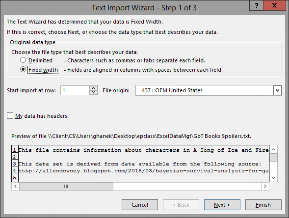
Step6. To change the file type to match the portion to import,

Click the Delimited radio button

Step7. Scroll down in the Preview portion of the dialog box, until you see the comma-separated data beginning on line 28.

Notice that the file GoT Books Spoilers.txt contains a title row. Since the worksheet does not have one yet, we will want to import the title row.

Step8. To start the import at the desired row, in the "Start import at row:" field,

Double-Click the value, type: 28

Step9. To confirm the settings,

Click

This part of the wizard allows the selection of the delimiter(s) that separates the columns of data. Tab is the default, which is not correct for this particular file. Let's change the settings to reflect the correct delimiter, commas.

Step10. To change the delimiter settings,

Click the Tab checkbox, Click the Comma checkbox

The Tab control is toggled off, and the Comma control is toggled on. The Preview pane also updates to reflect how the data will be split into columns.

Step11. To accept the these settings,

Click

This part of the wizard allows us to set the data format for each column. We will leave all of the fields as General for the most flexibility.

Step12. To complete the data import,

Click

The Import Data dialog box appears, asking where to place the data:

We can either put the data directly into the existing worksheet or into a new worksheet.

We will insert the data in this worksheet, beginning in cell A1, which is the current default setting. We do not need to make further changes in this dialog box.

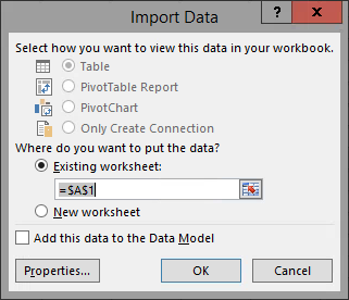
Step13. To complete the import,

Click

The data imports into a new worksheet in the workbook.

Step14. Save the workbook, Spoilers Backup.xlsx.

The file with the freshly imported data is now saved safely.

Next we want to make the "non-backup" copy of this file, so we can begin the data cleaning process.

Step15. Save the workbook as Spoilers.xlsx.

Now we can begin the process of examining and cleaning the imported data. First, let's see how to easily examine rows which are very far apart from each other.

Splitting Worksheets

When you are working with larger data sets on a spreadsheet, it may be helpful to view different areas of the same sheet at the same time. Splitting the worksheet enables separate scroll bars for each of the sheet's sections created by the split.

The split will occur immediately above the location of the active cell.

We can use the split to examine how the data is arranged overall (e.g., are there any entirely blank rows or columns), and also aspects of specific rows of data.

Step1. Scroll down the worksheet, to the entry for Arys Oakheart.

Step2. To activate that cell,

Click in cell A58

Step1. Switch to the View command tab.

Step2. To split the worksheet, in the Window group,

Click

The horizontal split bar appears. Row 57 is just above the horizontal split bar.

NOTE: If the cursor is not positioned in the first column, you will get a 4-way split with the window divided into four sections.

Step3. To scroll in the lower section,

Click in the bottom half of the window and scroll until row 128 (Catelyn Tully) is just below the split bar

Now it is easy to visually compare characters with allegiance to the House of Stark which are several rows apart on this worksheet.

Step4. Scroll through the data, and look for any completely blank rows or columns in the data set.

The data in the Allegiance column in particular suffers from inconsistent data entry. Multiple people conducted the data entry for this set, without agreeing on consistent values. That means there is variation in values that perhaps should be the same, which will cause problems in trying to analyze the data accurately. Later in this workshop we will see how to make data entry easier to perform and more consistent.

NOTE: To move the split bar, place the cursor over the bar until you see a cursor shape with vertical arrows, then press and drag the bar to a desired location.

The split can toggle on and off. Before we move on, let's remove the split.

Step5. To remove the split, on the View tab of the Ribbon,

Click

The split is toggled off, and we are back toward the top of the data, with row 58 visible. Now let's begin the next step of data cleaning.

Using Find and Replace to Change Data

Now we have confirmed the first few core steps of cleaning data. We have imported the data, made a backup workbook of the unmodified data, and we have verified our data set doesn't have any completely blank rows or columns within it. Now we want to change the data recorded about alleged character gender to use category words instead of the numeric code currently displayed. We can use the Find and Replace feature to do this.

Step1. Scroll to first row of the data set.

We want to select the entire column where we will be doing the Find and Replace, to restrict its action to that column.

Step2. To select the desired data,

Click the column G header

The entire column G is selected.

In Excel 2016 for Windows, the Find and Replace feature is available from the Home tab.

Step3. Switch to the Home tab on the Ribbon.

Step4. To locate the Find and Replace feature, in the Editing group,

Click

NOTE for MacOS Users: To activate the Find and Replace feature, on the Menu bar, Click Edit, Point Find, Click Replace...

Step5. To activate the Find and Replace feature,

Click Replace...

The Find and Replace dialog box appears.

In column G only, we want to change all 1s to be the binary gender category Male, and we want to change all the 0s to be the binary gender category Female.

Step6. To indicate the initial data to be found, in the Find what: field, type:

1

Step7. To indicate the initial replacement string,

Click in the "Replace with:" field, type: Male

Now, we wish to restrict where Excel will make such changes. By specifying some more options, we can restrict the replacement to only occur within the selected column. Let's see how to do this.

Step8. To reveal the options, in the Find and Replace dialog box,

Click

NOTE for MacOS Users: The controls are already visible.

The dialog box expands, revealing more controls. We want to conduct the replacement by columns, not rows, and if we specify an exact match of the cell contents, the replacement won't occur in unexpected places.

Step9. To search by columns, in the Search: drop-down,

Click By Columns

Step10. To ensure only an integer 1 is targeted,

Click the "Match entire cell contents" checkbox

Now the Find and Replace will be more restrictive, and we can replace all instances within the selected data.

Step11. To replace all of the 1s with the word Male,

Click

A message appears, informing you 760 replacements were made.

Step12. To dismiss the message,

Click

The Find and Replace dialog box remains open, and the entire column G is still selected.

Let's perform our second replacement now, finding all zeros and replacing them with the binary gender category Female.

Step13. To indicate the initial data to be found, in the Find what: field, type:

0

Step14. To indicate the initial replacement string, in the Replace with: field, type:

Click in the "Replace with:" field, type: Female

All of the prior options are still active.

Step15. To replace all of the 0s with the word Female,

Click

A message appears, informing you 157 replacements were made.

Step16. To dismiss the message,

Click

The Find and Replace dialog box remains open, and the entire column G is still selected. Now we can close the dialog box.

Step17. To close the dialog box,

Click

Step18. Save the workbook, Spoilers.xlsx.

Now let's use a different data set, and explore some other ways we can manipulate data sets in Excel.

Refining the Titanic Passenger List

Our next dataset contains information about the Titanic passenger list. Currently, the data is distributed across three worksheets in a workbook. Our task will combine the data into a single worksheet, and then make further changes to the data.

This dataset was obtained from the Department of Biostatistics Vanderbilt University.

The data is grouped by worksheet according to the passenger class (1st class, 2nd class,...) of the individuals, and we want to create a single worksheet containing all of the passengers data, so that certain kinds of analysis will be easier and more complete.

Let's open the workbook, TitanicList.xlsx, containing the data.

Step1. To open the desired workbook, press:

Control key+o, Click,
Double-Click TitanicList.xlsx

NOTE for MacOS Users: To open the desired workbook, press: Command key+o, Click On My Mac, Double-Click TitanicList.xlsx.

The workbook opens to the About worksheet. We want to combine all of the data safely. Let's make a copy of one of the worksheets, rename it, and then add copies of the other data to it, to create the single worksheet containing all of the data.

Copying a Worksheet

Since additional worksheets can be added or deleted easily, copying entire worksheets can be an efficient way to experiment with data without risk. Always make a copy of a worksheet before doing something that could result in an accidental or undesirable change to data.

Step1. To switch to the 1st Class worksheet,

Click the 1st Class worksheet tab

Step2. To begin making a copy of the worksheet,

Right-Click the 1st Class worksheet tab,
Click Move or Copy...

NOTE for MacOS Users: To begin making a copy of the worksheet, press Control key+Click the 1st Class worksheet tab, Click Move or Copy...

The Move or Copy dialog box opens:

We must specify a destination workbook, either a new workbook or any open workbook. By default, the current workbook is selected as the destination. Since this is where we want to keep our copy, we will accept the default. We must also specify the location that the worksheet will be copied to in relation to the order of the other worksheets in the destination workbook.

First, we will specify that we want to copy the worksheet.

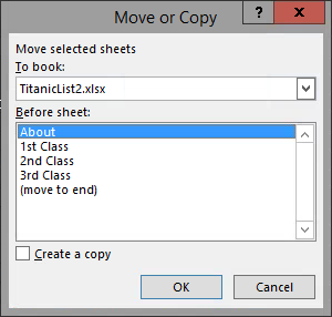
Step3. To select the "Create a copy" option,

Click the "Create a copy" checkbox

Step4. To copy the 1st Class worksheet to the end of the other worksheets, in the Before sheet field,

Click (move to end)

Step5. To complete the process,

Click

A copy of the 1st Class worksheet, named 1st Class (2), has been inserted into the workbook and is now the active worksheet. Let's rename it, to better reflect the actual contents it will contain.

Modifying a Worksheet Tab

We can give any worksheet a different name. Up to 31 characters are allowed in a sheet name. It is a good idea to keep the sheet names short and concise so that we can see more available tabs at the bottom of the workbook.

Step1. To select the worksheet tab name,

Double-Click the 1st Class (2) worksheet tab

Step2. To rename the tab, type:

AllPass Enter

The sheet tab shortcut menu contains a Tab Color command. Let's make this sheet a different color to make it easier to identify the worksheet copy.

Step3. To change the tab color,

Right-Click the AllPass worksheet tab
Point to Tab Color..., Clickany color

The active tab is white, except for a line of the selected color beneath the sheet name. The inactive sheet tabs are always displayed in full color.

Step4. Save the workbook, TitanicList.xlsx.

Now that we have made a duplicate worksheet with the data, we can continue working with this data range.

We already used the Consolidate feature today to summarize data from multiple worksheets. However, to combine all of the passenger data, we don't want to apply any summarizing function to the result, so Consolidate will not be a good option for this task. Instead, we will use a fast method for selecting a large range of data, then copy and paste that into the desired location.

Selecting the Current Region

When working with large data sets, we may want to copy the data itself, without making an entire copy of the worksheet. For some data, it may be fine to use a simple selection followed by copy and paste. For large or very large data sets, this may be impractical, as sometimes Excel can scroll with surprising speed when you are using the mouse to select data. However, Excel has a feature which makes selecting a large, well-structured chunk of data very easy to do, accurately.

If your data is in a range which has no blank rows or columns within the data itself, and the active cell is within that range, that range is considered the Current Region. The Current Region will extend to the right until Excel encounters a blank column, and then it will continue down until there is an entire blank row.

We will select the Current Region on the other two worksheets, then copy and paste the result into the AllPass worksheet to create our full dataset.

Let's see how to do this. We'll begin by copying the data from the 2nd Class worksheet.

Step1. To move to the desired worksheet,

Click the 2nd Class worksheet tab

The active cell is cell A1 on the 2nd Class worksheet. Now we will select the Current Region on this worksheet.

Step1. To begin to select the Current Region, on the Ribbon,

Click, Click Go To Special...

NOTE for MacOS Users: To activate the Find and Replace feature, on the Menu bar, Click Edit, Point Find, Click Go To..., Click Special...

The Go To Special dialog box opens:

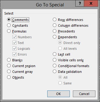
Step2. To select the Current Region,

Click the Current region radio button, Click

The entire region of data on the 2nd Class worksheet is selected. Now we will copy that selection and paste it under the existing data on the AllPass worksheet.

Step3. To copy the current selection, press:

Control key+c

A copied selection marquee appears around the data. Now we'll move to the destination worksheet, AllPass.

Step4. To move to the desired worksheet,

Click the AllPass worksheet tab

We want to paste our copied data under this existing data. We could scroll downward to do this, but there is a more efficient way to move the active cell from cell A1 to where we want it. Let's see how to do this.

Step5. To move the active cell to be under the last row of data, press:

Control key+Down Arrow key, and then press: Down Arrow key

NOTE for MacOS Users: To move the active cell to be under the last row of data, press: Command key+Down Arrow key, and then press: Down Arrow key.

The active cell is now cell A325. Now we can paste our selected data where we want it.

Step6. To paste the selected data, press:

Control key+v

The data is pasted under the existing data. Our selection had also included the label row, and it appears in the middle of the combined data now.

We can use the Remove Duplicates feature later, to remove the unwanted labels. For now, we want to perform similar actions to move the 3rd Class passengers data to this worksheet. This time, we'll use a keyboard shortcut to select the Current Region.

Step7. To move to the desired worksheet,

Click the 3rd Class worksheet tab

The active cell is cell A1 on the 3rd Class worksheet. Now we will select the Current Region on this worksheet, using just the keyboard.

Step8. To select the Current Region, press:

Control key+Shift key+*

NOTE for MacOS Users: To select the Current Region, press: Shift key+Control key+Spacebar.

The entire region of data on the 3rd Class worksheet is selected. Now we will copy that selection and paste it under the existing data on the AllPass worksheet.

Step9. To copy the current selection, press:

Control key+c

A copied selection marquee appears around the data. Now we'll move to the destination worksheet, AllPass.

Step10. To move to the desired worksheet,

Click the AllPass worksheet tab

We want to paste our copied data under this existing data.

Step11. To move the active cell to be under the last row of data, press:

Control key+Down Arrow key, and then press: Down Arrow key

NOTE for MacOS Users: To move the active cell to be under the last row of data, press: Command key+Down Arrow key, and then press: Down Arrow key.

The active cell is now cell A603. Now we can paste our selected data where we want it.

Step12. To paste the selected data, press:

Control key+v

The data is pasted under the existing data. Now we have two extra rows with the column labels information in this data. Let's save our work, and then remove those extra rows.

Step13. Save the workbook, TitanicList.xlsx.

Now we will use the Remove Duplicates feature to remove the extra label rows.

Removing Duplicates

When we remove duplicate values in Excel, we permanently delete duplicate values. The duplicate value is one where all specified values in the row exactly match all the same specified values in another row. The Remove Duplicates feature permits selection of columns for the specific data to be examined for duplicates. The initial row will be retained, and any other duplicate rows will be deleted. Obviously, this feature can be dangerous to data, so it is a good idea to save your workbook, as we have, before using this feature.

Step1. Switch to the Data command tab on the Ribbon.

There is currently a large chunk of data selected, and if we try to remove duplicates, that will be attempted only in the selection. We want the search for duplicates to occur across all of the data, so we need to change the current selection.

Step2. To select the Current Region, press:

Control key+Shift key+*

NOTE for MacOS Users: To select the Current Region, press: Shift key+Control key+Spacebar.

Step3. To begin to remove the duplicate rows, in the Data Tools group,

Click

The Remove Duplicates dialog box opens.

We will accept the default selection of all of the columns. However, we have an interesting situation where the duplicate rows to be removed actually match the header row. If we were to remove the duplicates right now, the second extra row of labels would be retained, and only the third one would be deleted. We want to delete both of the extra label rows at once. To do so, we will have to actually turn off the indication that the data has a header row, which is an unusual situation.

NOTE for MacOS Users: The behavior of Remove Duplicates is different. The confirmation of duplicates found is displayed before you actually change the data. To remove both duplicate rows, Click Remove Duplicates.

Step4. To permit a duplicate match to the header row,

Click the "My data has headers" checkbox

Step5. To remove the duplicate rows,

Click

A message box appears, indicating 2 duplicate values have been found and deleted from the range.

Step6. To close the message,

Click

Let's examine the results before we save the workbook again. We can view multiple worksheets at once to visually compare them.

Let's see how to do this.

Tiling Multiple Worksheets

Just as splitting a worksheet allows comparison of content in different areas of one sheet, tiling worksheets can enable the comparison of content in different worksheets whether they are in the same workbook or in different workbooks.

Let's tile the AllPass and 2ndClass worksheets for ease of comparison. When comparing two worksheets from the same workbook, we must first create a new window.

Step1. To create a new window for viewing, on the Ribbon,

Click the View tab, Click

NOTE for MacOS Users: To create a new window for viewing, on the Menu bar, Click Window, Click New Window.

It may seem that nothing much happened, but if you look at the title bar at the top of the window, you will see a number after the file name. We are looking at TitanicList.xlsx:2. Our goal in this exercise is to compare the original version of the 2ndClass worksheet with the AllPass worksheet data we have modified.

Step2. To select the 2nd Class worksheet at the bottom of this window,

Click the 2nd Class worksheet tab

We can use the Switch Windows button to switch between the two windows we now have.

Step3. Switch to the View tab again, if necessary.

Step4. To switch windows, in the Window group,

Click, Click TitanicList.xlsx:1

NOTE for MacOS Users: To switch windows, on the Menu bar, Click Window, Click Arrange.

In this window the active sheet is AllPass. But we would like to view these two worksheets without switching.

Step5. To view both worksheets in the same window, in the Window group,

Click

NOTE for MacOS Users: The options presented on the Ribbon are Tiled, Horizontal, Vertical, and Cascade. To restrict the windows being arranged, Click ‘Windows of active workbook".

The Compare Side by Side dialog box appears.

Because other workbooks open, we must select the other window which we want to compare side by side.

Step6. To select the desired window,

Click TitanicList.xlsx:2, Click

We see both worksheets with their own Ribbon, and they are currently arranged one over top the other.

NOTE: In Microsoft Excel 2016 for Windows, workbooks are shown as separate Excel windows with their own Ribbon, instead of multiple windows inside of a single Excel window. This means you will be able to display worksheets on different monitors.

Step7. Use the scroll bar to move to a different area of the active worksheet.

Notice that as one window scrolls, the other window scrolls as well. When two worksheets are displayed side by side, Synchronous Scrolling is enabled. We will turn this off in order that we may scroll the two windows independently.

NOTE for MacOS Users: This feature is not available in Excel 2016 for Mac. The windows will scroll independently.

Step8. To turn off Synchronous Scrolling, in the Window group,

Click

We want to verify the last entry on the 2nd Class worksheet matches the one in the AllPass worksheet.

Step9. To verify the last entry on the 2nd Class worksheet, in the TitanicList.xlsx:2 window, press:

Control key+Down Arrow key

NOTE for MacOS Users: To verify the last entry on the 2nd Class worksheet, in the TitanicList.xlsx:2 window, press: Command key+Down Arrow key.

Step10. Scroll to row 601in the AllPass worksheet, in the TitanicList.xlsx:1 window, to verify.

Step11. Scroll in both windows to make certain only the extra duplicate label rows were deleted. The other duplicate was at row 324.

Once we have verified that only the desired data was deleted, we can close the second window displaying the workbook.

Step12. Close the TitanicList.xlsx:2 window.

The TitanicList.xlsx workbook remains open.

Step13. Save the workbook, TitanicList.xlsx.

Now we can perform other modification to the range of data on the AllPass worksheet.