Introducing PivotTables

As data becomes more sophisticated, PivotTables can be used to analyze data and to help you make more wise decisions. A PivotTable report is a flexible report generated from a data source that quickly summarizes, organizes, and compares large amounts of data in a worksheet. The source data can reside in an Excel worksheet or in an external data file. Rows and columns may be rotated in a PivotTable to allow different views of the same data. The ability to "pivot" the dimensions of the table—for example, to transpose column headings to row positions, gives the PivotTable its name.

PivotTables help to answer questions you may have about your data. If your question sounds like "What is the [summary of variable] for each [category]?", then a PivotTable may be the correct tool to help you answer that rapidly.

Here are some other example questions a PivotTable might answer:

• How many employees does each department have?
• How much total salary is paid by each department?
• What's the median salary for each department?

The data on which the PivotTable is based is called the source data. Fields of information can be placed in Row or Column areas to organize the data. The Values area generally contains summarized numeric values. If there are no numeric data fields, a PivotTable can still provide a frequency count of data, for example student ID numbers. The Filter area fields are displayed as top-level report filters at the top of the PivotTable.

Here is an example of a PivotTable:

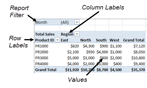
Tables can be imported from same or different data sources or imported simultaneously from a relational database. In an Excel PivotTable, we can take thousands of rows of data and quickly organize and rearrange the data to see different perspectives. Field drop-down arrows allow us to view all or portions of the data.

Creating a PivotTable

Before creating a PivotTable, the data must be organized into columns and rows, have column headings, and include no blank rows in the data. Since our data is organized in columns and rows with column headings, we can easily turn this information into a PivotTable report that will be useful at a glance. We want to be able to view total expenses and to select any quarter to see expenses for any particular category.

The PivotTable will appear in this final format:

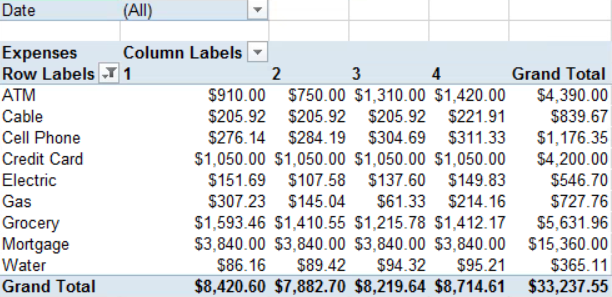
It is easier to maintain source data by first using Excel's Table feature. By converting the data to a table first, data that may be added in new rows or columns later will be automatically included in the PivotTable when it is refreshed or updated. Therefore, this is a real advantage since you won't have to remember to manually adjust the data range every time the data source changes.

To begin, we must first select a cell within the Transactions data.

Step1. Verify that a cell within the data is selected.

Now we are ready to create the PivotTable.

Step2. Switch to the Insert tab.

In Microsoft Excel there is an option to insert "Recommended PivotTables." By clicking any PivotTable layout to get a preview, you can choose the one that shows the data you want. Excel will place the PivotTable on a new worksheet. This is a quick way to get started, and you can still add and rearrange fields to the PivotTable layout any way you want.

For this PivotTable, we will insert a PivotTable and create the layout from scratch.

Step3. To open the Create PivotTable dialog box,

Click

You see the Create PivotTable dialog box:

Excel recognizes the table range, which we will accept.

We can place the PivotTable in a new worksheet or in the existing worksheet. If we choose Existing Worksheet, then we must specify the exact cell location for the PivotTable. We will place the PivotTable in a new worksheet.

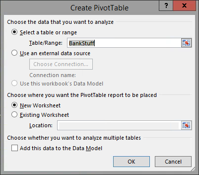
Step4. Verify that the New Worksheet radio button is selected.

Step5. To continue,

Click

Sheet 3 is now the active sheet which gives us a space to lay out the fields for our PivotTable. There is a blank table layout on the left side of the new sheet and a field list on the far right side of the sheet. Each field from the table appears in the field list accompanied by a preceding checkbox.

NOTE: The PivotTable Field List is normally docked on the right side of the window. However, you can drag the title bar to move it anywhere on the worksheet. If you Click a cell outside the PivotTable placeholder area, the PivotTable Field List will be hidden.

Before we design the PivotTable, let's rename the worksheet.

Step6. To name the worksheet tab,

Double-Click the Sheet# worksheet tab

Step7. To rename the tab, type:

Banking PivotTable Enter

Now we will arrange the fields.

There are multiple techniques for laying out a PivotTable:

• Press & Drag the fields from the field list to one of the four boxes in the Areas Section below the field list.
• Right-click a field name and choose its position in the PivotTable from the drop-down list.
• Click the checkbox of each field to be included and allow Excel to give it a default location in the PivotTable. This may require modification later.

We will use the Press & Drag method to place the fields in the appropriate boxes of the Areas section.

Step8. To select Category as the source for Row Labels, from the Field List,

Press & Drag Category to the Rows area

The layout should look like this:

The table begins to take shape in the worksheet with row headers - one row for each separate value in the Category column.

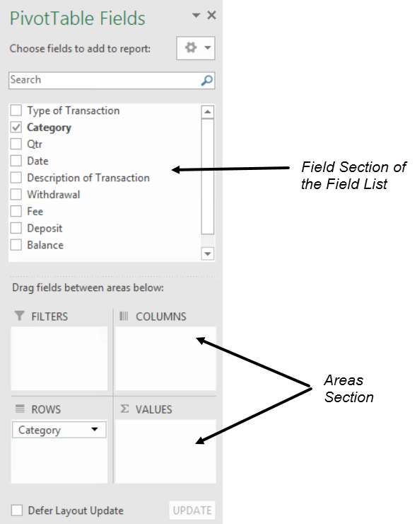
Step9. To make Qtr the source for Column Labels, from the Field List,

Press & Drag Qtr to the Columns area

The PivotTable now contains a column for each quarter.

Step10. To make Date the Report Filter field, from the Field List,

Press & Drag Date to the Filters area

Positioning Date as the Report Filter enables us to filter the table by different dates as necessary. A PivotTable does not have to have a Report Filter.

Step11. To provide data about withdrawals as the summarized information in this table, from the Field List,

Press & Drag Withdrawal to the Values area

The layout areas are set:

Notice that we see a count of the withdrawals. Instead, we would like to see the sum of withdrawals; therefore, we will change the function in the Values box.

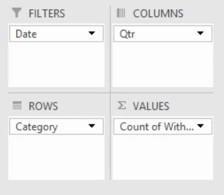
Step12. To open the Value Field settings window, in the Values box,

Click,Click Value Field Settings...

The Value Field Settings dialog box opens:

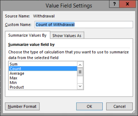
13. To change the function, in the "Summarize value field by" section,

Click Sum

Step14. To change the name of the field, in the Custom Name field,

Press & Drag the text, type: Expenses

Step15. To display the expense amounts as currency,

Click, Click Currency

NOTE for MacOS Users: The correct button is labeled "Number...".

Step16. To finish modifying the field settings,

Click, Click

The sums of all of the withdrawals now appear.

Step17. Save the workbook.

Pivoting the PivotTable

Currently, this PivotTable has Category in the Rows area, and Qtr in the Columns area. We can change how this data is = displayed in the PivotTable by "pivoting" or swapping the data in Rows with the data in Columns. This will still use the same data, but present it differently.

Let's see how to do this now.

Step1. To move the location of the Category data, in the Areas section,

Press & Drag Category from the Rows area to the Columns area

The PivotTable changes drastically, stretching out horizontally. Let's complete the pivoting of this data by moving the Qtr data, as well.

Step2. To move the location of the Qtr data, in the Areas section,

Press & Drag Qtr from the Columns area to the Rows area

Now the PivotTable is displaying the summary data again, but the Rows and Columns have been swapped. While the data is still accurate, the older view presented it in a more compact and slightly easier to understand way. Let's pivot the view back to what it was displaying previously.

Step3. To move the location of the Category data, in the Areas section,

Press & Drag Category from the Columns area to the Rows area

Step4. To move the location of the Qtr data, in the Areas section,

Press & Drag Qtr from the Rows area to the Columns area

The PivotTable is restored to how it appeared previously.

Filtering Data

PivotTables offer much flexibility in viewing data. We can hide data by using the column or row fields to display specific quarters or categories. By using the Report Filter drop-down list, we can further filter the information.

The "A Beginning Balance" and "Paycheck" categories are not withdrawals so we will hide those categories.

Step1. To deselect these categories, in the Row Labels drop-down box, in the PivotTable,

Click, Click the "A Beginning Balance" checkbox,
Click the Paycheck checkbox

Step2. To close the dialog box,

Click

Those categories are removed from the PivotTable.

Drilling Into the PivotTable Data

By double-clicking a value, we can see the hidden details behind any one particular value in the PivotTable.

Let's look at the Cable expenses from the second quarter.

Step1. To view the details underlying a value, in the PivotTable,

Double-Click cell C6

Excel copies the detail figures to a new worksheet and displays the data underlying that cell.

NOTE: To learn more on how to create and manipulate PivotTables, consider attending the workshop Excel 2016: Analyzing Data with Pivot Tables.

Linking Data to Another Worksheet

Earlier, we copied and pasted data from one worksheet to a new worksheet, to create a single list of the Titanic passengers. What we pasted was static data; it was a picture of the information at the time we copied it. Excel also allows us to create links between worksheets so that as data in the source worksheet changes, the linked data updates to reflect the changes, as well.

Let's see how to link the expenditures for third and fourth quarters from this PivotTable to cells on the AutoFill worksheet.

Step1. Switch to the Banking PivotTable worksheet.

Step2. To select the cells to copy, in the PivotTable worksheet,

Press & Drag cells D5 through E14

Step3. To copy the displayed cells to the clipboard, on the keyboard, press:

Control key+c

Step4. To activate the AutoFill worksheet tab,

Click the AutoFill worksheet tab

Step5. To indicate where to place the data,

Click cell B19

We will link the data using a Paste Special command, Paste Link.

Step6. To link the data, on the Home tab of the Ribbon,

Click, Click

NOTE for MacOS Users: The options have slightly different icons, and visible labels.

The category totals are pasted and linked into the worksheet.

Step7. To view the linked reference in cell B19,

Click cell B19

You can see the linked reference in the formula bar: =‘Banking PivotTable'!D5. It basically says that this cell contains the contents of cell D5 on the Banking PivotTable worksheet. You could also type this formula into the cell. Linking to a cell in a separate workbook requires the addition of the workbook name to the syntax such as: =‘[WorkbookName]PivotTable'!D5.

NOTE: If the worksheet name contains spaces, you will see single quotes around the sheet name. If neither the workbook name nor the worksheet name contains a space, the single quotes are not necessary.

Refreshing PivotTable Data

Outside of this workshop, data often changes, sometimes as we are working to analyze it. Pasting a link from one chunk of data to another will cause that linked data to update and reflect any changes. Because PivotTables are created using a snapshot of the data source, any changes in data values the PivotTable will need to be updated to reflect the new values. This process of updating data is called refreshing.

Let's change some data in the Transactions worksheet, and see how that change may ripple to other worksheets in this workbook.

Step1. Switch to the Transactions worksheet.

Step2. Change the value for the last ATM Withdrawal on 25-Dec to be $600.00.

The value changes in the Transactions worksheet. With that great a change to the ATM values, the ATM subtotal for the 4th Quarter should now be just over $1,400. Let's see where that new value is and isn't reflected in the other worksheets using that as source data, the AutoFill worksheet and the Banking PivotTable worksheet.

Step3. Switch to the Autofill worksheet.

The ATM values for the 4th Quarter remain unchanged. The data we are looking at is linked to the BankingPivotTable worksheet. It also may not have changed. Let's see if it has.

Step4. Switch to the Banking PivotTable worksheet.

The PivotTable values remain unchanged, because PivotTables use a snapshot of the source data, by default. We can force the data to be updated in the PivotTable. Let's see how to do this.

Step5. To update the data used in the PivotTable,

Right-Click the PivotTable, Click Refresh

The value displayed for the ATM 4th Quarter is updated, to reflect the newest values. Now let's verify this matches the linked data on the AutoFill worksheet.

Step6. Switch to the Autofill worksheet.

The linked data now matches the data being displayed in the PivotTable.

NOTE: When linking data between workbooks, be careful when changing names or locations of related linked files. Also, links are normally updated automatically when the source and destination workbooks are open on the same computer. If they are not both open, you may be alerted by the Trust Bar to update the links.

Step7. Save the workbook.

Now we have time to practice more using PivotTables. If you wish to do that, please move forward to the next section.

Step8. If you do not wish to take advantage of this opportunity, exit Excel.