Using the Auto Fill Feature

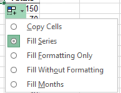
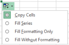
As you have seen, dragging the fill handle in a cell allows you to quickly fill or copy cells. You can also use the Auto Fill feature to create a series that is based on an interval between two selected values or create custom lists to make entering a particular sequence as easy as dragging the mouse.

Dragging the Fill Handle to Extend Data in Cells

Auto Fill normally increments recognizable time and date values when you drag the fill handle, even if you initially select one cell. If a selection contains both text and numeric values, the Auto Fill feature takes over and extends the numeric component while copying the text component.

Some examples of simple data series are shown below:

We will fill in additional labels and values in a budget worksheet for the last six months of the year by using Excel's Auto Fill feature.

We will first populate row 4 with column headings of abbreviations of the rest of the year.

First we must switch to the AutoFill worksheet.

Step1. Switch to the AutoFill worksheet.

Step2. To make B4 the active cell, if necessary,

Click cell B4

You see a small box, which is the fill handle, in the lower right corner of the border area.

Step3. To perform the Auto Fill operation,

Point to the fill handle in the lower right corner

You see:

The cursor changes to a thin, solid crosshairs plus symbol.

Step4. To create the heading series,

Press & Drag the fill handle to cell G4

When the mouse button is released, the labels for the last six months of a year are filled into cells B4 through G4.

NOTE: You can also reverse the order by simply dragging the fill handle either upward or to the left.

After we drag, an Auto Fill Options button appears:

This button will give us different options from which to choose.

Step5. To view the Auto Fill options,

Click the Auto Fill Options button

You see:

The Options menu shows the default as Fill Series since Excel knew to repeat the pattern of selected cells to fill the range.

Step6. To cancel the Options menu, press:

Esc key

Next, we will use the Auto Fill feature to drag a single value to the August column.

Step7. To select the ATM value for July,

Click cell B5

Step8. To perform the Auto Fill operation, in the lower right corner,

Point to the fill handle

Step9. To copy the value to C5,

Press & Drag the fill handle to cell C5

When the mouse button is released, Excel copies the contents of cell B5 to C5, and the Totals column reflects a change. Another options menu appears and gives us options from which to choose after we drag.

NOTE: When dragging single selected values, Excel normally copies them unless it recognizes time or date values. However, if you hold down the Control key while dragging, Excel extends the series with consecutive numbers. In other situations when Excel fills in a series, you can hold down the Control key to suppress Auto Fill and copy the selected values.

Step10. To view the Auto Fill options,

Click the Auto Fill Options button

You see:

If we were to change our choice to Fill Series on the Option menu, Excel would create the simple series of 151, 152, 153, etc.

Step11. To cancel the Options menu, press:

Esc key

There is an alternative method to copy and fill cells. After we select the range we want to fill, we will use the Fill options on the Home tab of the Ribbon to fill the August column with the range of July values.

Step12. To select the range for the August expenses,

Press & Drag the cell range C6:C13

Step13. To perform the Auto Fill operation, on the Home tab, in the Editing group,

Click, Click Right

The selected range, which is to the right of the existing content, is filled with those same values.

NOTE: The Fill menu allows content to be continued into adjacent cells in any direction. You will notice other options in the Fill menu that allow the user to fill cells across worksheets or to specify series options.

We will change the ATM and Gas values and then see how values will increment or decrement automatically when we use the Auto Fill feature.

Step14. To change the ATM value in cell C5,

Click cell C5, type: 140 Enter

Step15. To change the Gas value in cell C10,

Click cell C10, type: 130 Enter

Next we will select and copy both the July and August columns to maintain the same decrements and increments for the ATM and Gas values.

Step16. To select both July and August values,

Press & Drag the cell range B5:C13

Step17. To perform the Auto Fill operation,

Point to the fill handle, Press & Drag the fill handle to cells G5:G13

The data series is completed for July through December with the ATM and Gas expenses showing increasing and decreasing increments of $10.

Step18. To view the Auto Fill options,

Click the Auto Fill Options button

The Options menu now shows the default as Fill Series since Excel knew to repeat the pattern of selected cells when filling the range.

Step19. Cancel the Auto Fill Options menu.

NOTE for MacOS Users: Skip foward to the heading, "Creating a Custom List on MacOS".

Creating a Custom List on Windows

A custom list is useful when a particular sequence of data must be repeated in a worksheet. When the sequence is created, it can be entered in any range of cells by simply typing the first item in the series and then dragging the fill handle to complete the series. When you create a custom list, it is global within the Excel program on the computer on which it was created. Therefore, the list will be available for any spreadsheet on that computer until the custom list is deleted.

Since we will be using the same expense categories repeatedly in our worksheets, we will create a custom list. A list may be typed manually in the Custom Lists dialog box or imported from an existing cell range.

Our categories are already typed in the desired order in the worksheet, so we will select the range and import the entries rather than retyping them.

Step1. To select the category items,

Press & Drag the cell range A5:A13

Step2. To open the Excel Options dialog box,

Click the File tab, Click Options

Step3. To access the Advanced section of the Excel Options dialog box, in the left pane,

Click Advanced

Step4. To access the Custom Lists dialog box, near the bottom of the dialog box, in the General section,

Click

You see the Custom Lists dialog box.

We will import the selected categories as a custom list. The reference to the selected data range is already entered in the field. If we had not selected it prior to opening this dialog box, we would need to enter it here. Selecting the range first saves some effort.

Step5. To add the list to the Custom lists box,

Click

The list now appears as a new list in the Custom lists box with each entry listed separately.

NOTE: When adding or importing a new list by typing, be sure to type the items in the order that you want them to appear. List items are not case sensitive.

Step6. To close the dialog box and the Excel Options window,

Click, Click

The new custom list is added, and we are returned to the worksheet. Now we can type any item from this sequence in any cell and then simply drag the fill handle to fill in a range of cells. This list will be available within any workbook on this computer now.

Note for Windows Users: Skip foward to the heading, "Using a Custom List".

Creating a Custom List on MacOS

A custom list is useful when a particular sequence of data must be repeated in a worksheet. When the sequence is created, it can be entered in any range of cells by simply typing the first item in the series and then dragging the fill handle to complete the series. When you create a custom list, it is global within the Excel program on the computer on which it was created. Therefore, the list will be available for any spreadsheet on that computer until the custom list is deleted.

Since we will be using the same expense categories repeatedly in our worksheets, we will create a custom list. A list may be typed manually in the Custom Lists dialog box or imported from an existing cell range.

Our categories are already typed in the desired order in the worksheet, so we will select the range and import the entries rather than retyping them.

Step1. 1. To open the Excel Preferences, on the Menu bar,

Click Excel, Click Preferences...

Step2. To access the Custom Lists pane,

Click Custom Lists

You see the Custom Lists pane appear.

We will import the selected categories as a custom list. The reference to the selected data range still needs to be entered in the "Import list from cells:" field.

Step3. To enter the desired range into the "Import list from cells:" field,

Click, Press & Drag the cell range A5:A13,
Click

The range $A$5:$A$13 is in the "Import list from cells:" field.

Step4. To confirm adding the data in the selection to the List entries and Custom lists fields,

Click

The list now appears as a new list in the Custom lists box with each entry listed separately.

NOTE: When adding or importing a new list by typing, be sure to type the items in the order that you want them to appear. List items are not case sensitive.

Step5. To close the Custom Lists pane,

Click

The new custom list is added to this copy of Excel's Preferences, and we are returned to the worksheet. Now we can type any item from this sequence in any cell and then simply drag the fill handle to fill in a range of cells. This list will be available within any workbook on this computer now.

Let's see how this works.

Using a Custom List

We want to use this same list of expense categories in another location on the sheet.

Step1. To begin the data series,

Click cell A19, type: ATM Enter

NOTE: If we begin the series with a capital letter, Excel will extend the series with each item in the list beginning with a capital letter. Conversely, if we begin the series with a lowercase letter, Excel will extend the series with each item beginning with a lowercase letter.

Step2. To select the series beginning entry,

Click cell A19

Step3. To perform the Auto Fill operation,

Point to the fill handle, Press & Drag the fill handle to cell A27

The data series has been created with the custom list.

Step4. Deselect the column.

Step5. Save the workbook.

NOTE: Custom lists can be edited by going into the Custom Lists dialog box, selecting the list, and then deleting the entire list or modifying an entry in the list.

Creating Another Table

When a range of cells is made into a table, data in that table can be analyzed and managed independently of data in other areas of the worksheet. We can create a table from an empty range or from an existing range of data. The data can be easily filtered, summarized with a total row, and formatted.

Let's make this data range a table.

Step1. Switch to the Transactions worksheet tab.

Step2. Verify that a cell within the data range is the active cell.

Step3. To select the Insert tab, on the Ribbon,

Click the Insert tab

Step4. To create the table, in the Tables group,

Click

You see the Create Table dialog box. Excel guesses the intended range of cells for the table. If the range is incorrect, you can change the description. The dialog box also allows you to indicate the presence of a header row in the range.

Step5. Verify that the "My table has headers" checkbox is selected.

Step6. To complete the table creation,

Click

The range of cells now displays the default table style. The headings in row 1 display drop-down arrows for use in filtering the data. A new contextual tab appears on the Ribbon (on Windows, there is a Table Tools parent tab; on MacOS the new tab is simply labeled Table).

Step7. To deselect the table,

Click any cell in the table

Step8. Save the workbook.

Working with the Name Manager

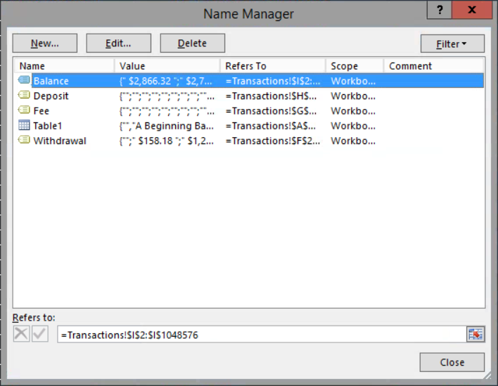
Cell ranges can be given names that are easy to remember and use in formulas. The table we just created was given a name, too. The Name Manager in Excel 2016 for Windows provides a convenient way to organize and edit all the names used in a workbook. Next, we will explore the Name Manager.

NOTE for MacOS Users: There is no Name Manager feature in Excel 2016 for Mac. Renaming the table may be accomplished using the Name Box on the Formula bar, or by using the Define Name button in the Formulas command tab.

Step1. To select the Formulas tab, on the Ribbon,

Click the Formulas tab

Step2. To open the Name Manager, in the Defined Names group,

Click

The Name Manager dialog box opens:

NOTE for MacOS Users: To open the Define Name dialog box, in the Defined Names group, Click Define Name button.

The New button in the Name Manager can be used to assign names, such as sales tax and interest rate, to values or to complex formulas or formulas that might be difficult to remember.

Each name used in the Transactions worksheet is listed. The Refers To column may help differentiate between the uses, if a name should be used on multiple sheets. The table we just created is named Table 1 by default. Let's give it a more descriptive name.

Step3. To select the default name for the table,

Click Table1

NOTE for MacOS Users: Skip the next step.

Step4. To open the Edit Name dialog box, at the top of the Name Manager,

Click

The Edit Name dialog box opens with the default name, Table1, selected. Notice that we are allowed to change the name or add a comment, but the Scope and Refers To fields are unavailable. When creating a new name from the Name Manager, the Scope of the name can be set to the current worksheet or to the entire workbook.

Step5. To change the name, type:

BankStuff, Click

The name Balance was applied to cells in that worksheet, but the name is not actually being used in any formulas. We can select that name and safely delete it, since no formulas depend on its existence.

Step6. To select the first instance of the name Balance, in the list of names,

Click Balance

Step7. To delete the selected name,

Click

You are prompted to confirm this action.

Step8. To confirm that the name should be deleted,

Click

Step9. To close the Name Manager,

Click

Step10. Save the workbook.

Inserting a New Row

We will enter a new record manually and look at a couple of text data entry features that can assist with repetitive entries. One advantage of working with tables in Excel is that the heading row labels will replace the column letters as you scroll toward the bottom of the sheet. This has an effect of freezing panes without actually performing that step. As we scroll down the worksheet, the heading row will stay in view.

Let's add a new deposit record, beginning in the first column of row 192.

Step1. To navigate to row 192, using the vertical scroll bar,

scroll to the bottom of the table

Notice that the table headers appear instead of the column letters.

Step2. To begin the new record, in the first column,

Click in cell A192

Step3. To enter the transaction, type:

Direct Deposit Tab key

The AutoComplete feature for text entry activated, and made the text match the case of prior entries in the column. Also, by adding a new row of data to the table, the current region for the named range has been automatically updated.

We will view the validation list that has already been created for Column B.

Step4. To view the drop-down validation list, in the second column,

Click

All of the current categories are listed. We could choose a category from this drop-down list, but we will see how to enter data in the cell using the AutoComplete feature.

NOTE for MacOS Users: To enter the desired Category, in the drop-down list, Click Paycheck. Then skip ahead to Step 7 below.

Step5. To cancel the drop-down list, press:

Esc key

Excel's AutoComplete feature will recognize the category as paycheck once we begin typing, since that text entry has already been used in a previous record.

Step6. To begin typing paycheck, type:

p

Excel suggests paycheck as the text for this cell. We can press Tab, Enter, or an arrow key to go to the next cell and accept Excel's completion.

Step7. To accept the paycheck entry and go to the next cell, press:

Tab key

Excel 2016 for Windows' AutoCorrect feature changed "paycheck" to be "Paycheck". This makes it match exactly with the other entries in this column.

NOTE: If, for some reason, AutoComplete gets in the way, you can turn it off by going to Excel Options in the Backstage, Click the Advanced category button, and clear the "Enable AutoComplete for Cell Values" checkbox.

Step8. To enter the quarter, type:

4 Tab key

Step9. To enter the date, in the Date column, type:

12-30-16 Tab key

You see a warning appear about the date:

Since a validation rule has been set for this column to give us a warning if the date doesn't fall within five previous days of the current date, Excel asks us to confirm the entry.

NOTE: The validation criteria for this column is as follows: the Start date is =TODAY()-5 and the End date is =TODAY().

Step10. To accept the date,

Click

Next we will look at the Pick From Drop-down List... feature which can also assist us with text data entry if we don't use validation criteria. This command will give us a list of all items in the current column from which to choose.

Step11. To choose the entry from a drop-down list, in the Description of Transaction column,

Right-Click the cell in row 192,
Click Pick From Drop-down List...

We can see all of the transaction descriptions listed in the drop-down list.

Step12. To select the Direct deposited option,

Click Direct deposited ,
press: Tab key Tab key Tab key

Step13. In the Deposit column, type:

2723.19 Tab key

Excel extends the Balance formula in the Table automatically, so the new balance is calculated.

Adding a Total Row

Let's see how easily we can add a Total Row to the table.

Step1. To switch to the Design tab, on the Ribbon,

Click the Design tab

NOTE for MacOS Users: To switch to the Table command tab, on the Ribbon, Click the Table tab.

Step2. To add a Total row to the table, in the Table Style Options group,

Click the Total Row checkbox

The word Total was added to cell A193 and the result of a formula displays in the Balance column of row 193. By default, Excel will automatically calculate the far right column. We will alter the totals in the total row.

Step3. To select the Balance total, in the Balance column,

Click in row 193

Step4. To eliminate the Balance total,

Click, Click None

It might be helpful to know the total number of times we have paid fees.

Step5. To show the number of fees entered in this table, in the Fee column,

Click in row 193, Click, Click Count

There are 7 accrued fees.

Perhaps it would also be helpful to know the total of all withdrawals we have made. This may be useful when we filter certain categories.

Step6. To display total withdrawals, in the Total row, in the Withdrawal column,

Click in row 193, Click, Click Sum

The total withdrawals show $32,697.55. The formula bar shows the Subtotal function in place now in this cell: =Subtotal(109,[Withdrawal]). The first argument,109, represents the Sum function we chose for the calculation. The second argument, Withdrawal, is the name of the range being added.

Next we will see how to filter data.

Filtering Rows

To filter a table means to hide all of the rows except those that meet specified criteria. Excel tables have the filter feature turned on automatically as evidenced by the drop-down arrow next to each heading in row one.

Filtering can be turned on for other ranges that are not tables by:

• Choosing Sort/Filter from the Home command tab
• Choosing Sort/Filter from the Data command tab
• Right-clicking any cell in the range and choosing Filter

We will select a cell within the table and then use this feature to extract data from the table.

Drop-down arrows appear next to each column heading. We will set the category for grocery expenditures.

Step1. To select a specific type of Category, within the Category heading,

Click

NOTE: As long as the insertion point is positioned somewhere within the table, you will see the drop-down arrows for filtering without having to return to the beginning of the table.

A list of all the different categories appears. All appear to be selected.

Step2. To deselect all categories,

Click the (Select All) checkbox

All the category checkboxes are cleared.

Step3. To see only the Grocery records, in the category list,

Click the Grocery checkbox, Click

NOTE for MacOS Users: To see only the Grocery records, in the category list, Click the Grocery checkbox, then close the pane. To close the pane, Click.

The displayed rows change to only display the entries which have the Grocery category applied to them. Notice that all of the rows are hidden except those specified as Grocery in the Category column. The icon next to the grocery header has changed to indicate a filter has been applied there. Also, evidence of the filter appears in the lower left corner of the status bar.

Step4. To view the Totals row, if necessary,

scroll upward to view the Grocery records

The Totals row now shows the total for grocery expenditures.

Adding Additional Criteria

A search for data can be further refined by setting additional criteria within a different field. For example, suppose we were interested in finding out how much was spent on groceries in April. Since we have already selected all Grocery records, we need only to set a new criterion in the Date column.

Step1. To see a list of all dates, in the Date heading cell,

Click

Step2. To deselect all dates,

Click the (Select All) checkbox

Step3. To select the month of April,

Click the April checkbox

NOTE: Checkboxes for the individual April dates which have transactions would be revealed if the expansion control were to be toggled on. To activate the expansion control, Click.

Step4. To complete the selection,

Click

Three grocery records for April are displayed.

Using Custom Filters

Sometimes filtering criteria can be more difficult to describe. By using custom criteria, we gain a little more flexibility in building that description. We can filter values above or below a specified value, values within a range, two discrete values, or approximate matches. Wildcards (? or *) can also be used to filter in other ways. In a column's Filter drop-down menu, under the Data Filters item is an option for "Custom Filters...", which permits using them against the data.

Copying Filtered Results to a New Worksheet

We may want to work further with these transactions without the other entries which have been hidden by the filter. Let's see how to easily select, copy, and paste to another worksheet using only the visible data.

Let's first select just the April Grocery transactions.

Step1. To select the desired transactions,

Press & Drag the cell range B55:I59

The entire range is selected, including the hidden rows. If we copy this range, all of the rows within the selected ranges will be copied. However, we can use a special keyboard shortcut to select only the displayed rows.

Step2. To select only the displayed rows, press and hold:

Alt key+;

NOTE for MacOS Users: To select only the displayed rows, press and hold: Command key+Shift key+*.

Only the displayed rows are now selected.

Step3. To copy the selected rows, press:

Control key+c

The "marching ants" indicate that these rows are copied to the Office clipboard and are ready to be pasted. But we need a new sheet on which to place the information.

Step4. To insert a new worksheet, at the bottom of the sheet, to the right of the workbook tabs,

Click

A new worksheet appears. The cursor is in cell A1.

Step5. To paste the selection, press:

Control key+v

Step6. Expand the column widths, as necessary.

We will rename this worksheet.

Step7. To select the worksheet tab name,

Double-Click the Sheet# worksheet tab

Step8. To rename the tab, type:

April Enter

Now that we have captured the April Grocery entries on their own worksheet, let's return to the Transactions sheet and see how to remove the filtering and return the sheet to its original appearance.

Resetting Table Filters Rapidly

Filters for individual columns in a Table may be reset one at a time, but we can also rapidly reset all filtering which has been performed in a Table by simply removing and then restoring the filters. We can also remove the Total row from this table so it won't interfere with further possible analysis of the data.

Let's see how to do this.

Step1. Switch to the Transactions worksheet.

Step2. To disable the Total row, on the Design tab,

Click the Total Row checkbox

NOTE for MacOS Users: To disable the Total row, on the Table tab, Click the Total Row checkbox.

An Excel warning appears stating that turning off the total row may cause formulas or names to return unexpected results.

Step3. To continue,

Click

Step4. To quickly disable the filters and re-display all transactions,

Click the Data tab, Click

All records are displayed, and the Filter drop-downs disappear from all of the columns. These filters can be toggled on or off. By default, they are on when the Table is created. Let's restore their presence again.

Step5. To enable the column filters,

Click

Step6. Save the workbook.

The Transactions worksheet data should be back to its original state as a Table, plus the additional entry we had made.