Validating Data

The Data Validation feature allows rules which ensure that specific cells in a worksheet meet specified criteria or accept certain types of data, such as dates or whole numbers. We can also force users to select valid data from a list in a drop-down box. Excel can display a message that prompts users for correct entries and can even display an error alert when a user enters data incorrectly. 

Some important issues concerning data validation are:

• Data validation rules work best when users type data directly into cells.
• Data validation rules do not affect pre-existing data, but can be used to visually flag existing data which does not comply with those rules.
• If existing data is deleted, then the data validation rules will apply to those cells when the user enters new data, if the cells still have had the validation rules applied.
• It is too easy to overwrite a target cell's validation rule by copying and pasting data or using the drag fill handle to enter data.

Now we will open an existing workbook and create some validation rules to show how to minimize data entry errors.

Opening an Existing Workbook

To explore some more of Excel's data entry-related features, we will open a workbook called ManagingMyData.xlsx.

Step1. To begin to open a workbook, press:

Control key+o, Click Browse

Step2. To open the desired workbook,

Double-Click ManagingMyData.xlsx

Excel opens the workbook.

We will use the Validation worksheet to set up some validation rules when entering employee data.

Step1. To switch to the Validation worksheet, if necessary,

Click the Validation worksheet tab

The Validation worksheet contains two records that do not follow all the rules we plan to put in place for this sheet's data. Later, we will see how Excel's validation feature deals with this existing data, to see how to easily find such instances.

NOTE: If a cell contains a value or formula that Excel thinks may be an error, a triangle will appear in the top left corner of the cell; for example, Excel may assume that numbers should not be stored as text. To disable Error Checking, you can go to The Backstage, then open the Excel Options dialog box, Click Formulas in the left panel, and under the Error Checking category, disable the "Enable background error checking" checkbox. At any time, the background error checking tool can be enabled to locate cells that might contain errors.

NOTE for MacOS Users: To disable Error Checking, on the Menu bar, Click Excel, Click Preferences..., then Click Error Checking, and uncheck the "Turn on background error checking" checkbox in the Error Checking dialog box.

Specifying Data Validation Criteria

Validation rules can be mandatory or optional. If the rules are mandatory, Excel will refuse to accept an entry that does not meet the required standards. We can also set up advisory prompts in which the user will be prompted, but not forced, to enter particular kinds of data.

We will first select the range of cells where we want the criteria to apply, and leave some room for new hires to occur. Then we will set up a validation rule to limit the Employee ID to four characters.

Step1. To select the criteria range for the Employee ID,

Press & Drag cells A4 through A24

Step2. To view the Data tools, on the Ribbon,

Click the Data command tab

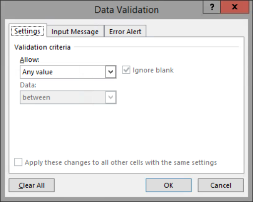
Step3. To access the Data Validation dialog box, in the Data Tools group,

Click

NOTE: Depending on the display settings of your machine, you may see a larger button.

You see the Data Validation dialog box:

The controls in the Settings tab will vary, depending upon the choices in the Allow drop-down box.

The following options are available in the Allow drop-down box:

We want to limit the Employee ID to four characters, so we will select the Text length option.

Specifying Text Length

When specifying text length, the field can be any data type. Text Length only creates a length requirement, not a requirement for the text itself.

We will make the text length four characters for the Employee ID column.

Step1. To select the Text length option, in the Allow drop-down box,

Click, Click Text length

Step2. To select a Data option, in the Data drop-down box,

Click, Click equal to, press: Tab key

Step3. To set the length to four characters, in the Length field, type:

4

The text length is set to four characters.

We also want to give the user specific information to guide the data entry process and avoid errors, so we will create an input message. Input messages are optional, but they are very useful.

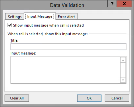
Step4. To view the input message options,

Click the Input Message tab

You should see:

Notice that the input message may be enabled or disabled by a checkbox. We can specify a title for the input message as well as the content of the message.Using a full sentence (or sentences) can help create more trust in the message.

Step5. To specify a title for the input message,

Click in the Title field, type: Employee ID Tab key

Step6. To specify the input message, in the Input message field, type:

Employee ID must be 4 digits long.

This message will be displayed as a comment beside the validated cell whenever the user selects the cell. Next we will set an error alert to specify the style of message that appears when an invalid value has been entered.

Step7. To specify an error alert,

Click the Error Alert tab

The following style choices are available:

We will leave the default Style setting at Stop to prevent an invalid entry for the Employee ID field.

Step8. Verify that the Style setting is set to Stop.

Step9. To create a title for the message,

Click in the Title field, type: Employee ID Tab key

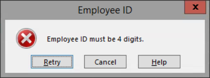
Step10. To create the message, in the Error message field, type:

Employee ID must be 4 digits.

Step11. To close the dialog box,

Click

A user must now enter four characters when entering the Employee ID in the range we specified. Notice that while the value in cell A4 breaks the rule we just created, Excel allows it since these validation rules do not affect pre-existing data. While data validation cannot force existing data to comply with validation rules, non-compliant data can be visually flagged easily, once the validation rules exist.

Specifying Date Criteria

The Date option allows us to specify a date range. We want to specify that hihre date entries must be on or before today's date.

To do this, let's first select the range of cells where we want the date criteria to apply. Then we will set up a validation rule to warn the user to enter a date on or before today's date.

Step1. To select the criteria range for the Hire Date,

Press & Drag cells D4 through D24

Step2. To open the dialog box, on the Ribbon,

Click

The Data Validation dialog box opens showing the last tab we selected. Let's return to the Settings tab.

Step3. To activate the Settings tab,

Click the Settings tab

Step4. To select the Date option, in the Allow drop-down box,

Click, Click Date

Step5. To select the operator, in the Data drop-down box,

Click, Click less than or equal to, press: Tab key

Step6. To set up the validation criteria, in the End date field, type:

=today()

Excel stores dates as sequential serial numbers so they can be used in calculations. This function returns the serial number of the current date and accepts no arguments. If you enter the function into a cell with the General format (the default), the resulting value is displayed in mm/dd/yyyy format. Remember to include the empty parentheses. Excel will convert this function to all caps.

We won't enter an input message this time, but we do want to set a warning that the hire date should be on or before today's date.

Step7. To specify an error alert,

Click the Error Alert tab

For the hire date, we will set a warning to allow a little more flexibility in entering this date. This will allow for a situation where an employee will be hired after today's date.

Step8. To change the Style to Warning, in the Style drop-down box,

Click, Click Warning

Step9. To create a title for the message,

Click in the Title field, type: Hire Date Tab key

Step10. To create the message, in the Error message field, type:

Hire date should be on or before today's date.

Step11. To accept these changes and close the dialog box,

Click

If a user tries to enter a date after today's date in the range specified, a warning will appear. The user will then have an opportunity to either continue and leave the date as entered, change the date, or cancel and start over with a different entry.

Creating a Drop-Down List

A common use of data validation is to create a drop-down list of items. The items may be entered directly into the Source control in the Settings tab of the Data Validation dialog box separated by commas, or for longer lists, a range for a list of items can be created on the worksheet and then entered in the dialog box.

Until now, we have applied validation rules directly to a range of cells. It is also possible to copy and paste validation rules. To show how this is done, we will set up a validation rule for a drop-down list for the Region field in one cell, and then copy this validation criteria to a range of cells.

Step1. To select the first cell under Region,

Click cell F4

Step2. To open the Data Validation dialog box, on the Ribbon,

Click

The Data Validation dialog box opens.

Step3. To activate the Settings tab,

Click the Settings tab

Step4. To select the List option, in the Allow drop-down field,

Click, Click List, press: Tab key

Step5. To specify the list items, in the Source field, type:

East, West, North, South

NOTE: Each item must be separated by a comma, but spaces are not required. A data range or a named range may also be specified here, using the appropriate reference syntax.

When we enter list items in this manner, they are case sensitive. If they are entered in the Source box with capital letters, then they will be displayed in the list and stored that way.

Step6. To specify an error alert,

Click the Error Alert tab

Step7. Verify that the Style setting is set to Stop.

NOTE: To allow users to type items that are not in the list, change the Error Alert to Warning or Information.

Step8. To create a title for the message,

Click in the Title field, type: Region Tab key

Step9. To create the message, in the Error message field, type:

As of 2000, region must be East, West, North, or South

Step10. To set the validation,

Click

The active cell displays a drop-down arrow. Users entering new records will be required to choose from the list one of the four validation criteria options.

Important Notes on Creating Drop-Down Lists

There are a few things to keep in mind when specifying data validation for a list in the Source box:

• Named ranges must be preceded by an equal (=) sign.
• Ranges specified as validation lists are not case sensitive.
• When providing a cell range in the Source box, the drop-down list will automatically be updated if any item in the list is modified.
• If the list is deleted from a specified range, then the items in the drop-down list for the validation range will not appear.

Copying and Pasting Validation Criteria

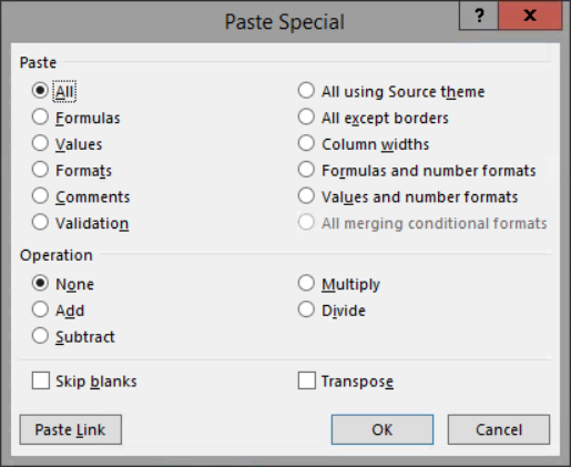
When performing a copy and paste, we may not always want to copy everything from the source range to the destination range. For example, we may not want to overwrite existing data or formulas with new data, but we may want to copy validation rules. The Paste Special dialog box gives us other options and allows more flexibility in controlling what is copied from the source range to the destination range.

Once validation criteria have been created, we can apply the same criteria to other cells without copying the data from the cells themselves. Let's see how to copy validation criteria to a new range for the Region field so that the same data validation rules for the drop-down list apply.

Step1. To select the validation criteria for Region, if necessary,

Click cell F4

Step2. To copy the cell, on the keyboard, press:

Control key+c

Step3. To select the cells to which we want to copy the validation criteria,

Press & Drag cells F5 through F24

We will open the Paste Special dialog box to control what we want to copy to the destination range.

Step4. Switch to the Home tab.

Step5. To open the Paste Special dialog box,

Click, Click Paste Special...

NOTE: The keyboard shortcut to open the Paste Special dialog box is Control key+Alt key+v.

NOTE for MacOS Users: The keyboard shortcut to open the Paste Special dialog box is Command key+Control key+v.

The Paste Special dialog box appears:

There are several paste options, which are explained:

Step6. To select the validation option,

Click the Validation radio button

Step7. To close the Paste Special dialog box,

Click

The validation criteria has been copied and pasted to the selected destination range.

NOTE: A Ctrl Options button will appear at the end of the selection, which will display additional paste options.

Step8. To discontinue the selection marquee, on the keyboard, press:

Esc key

Locating Cells with Existing Data Validation

We may want to find all of the cells on a worksheet that have data validation. We will see how to do this now.

Step1. To select all cells on a worksheet that are set up for data validation, on the Home tab, in the Editing group,

Click, Click Data Validation

NOTE for MacOS Users: To find all cells with data validation, on the Menu bar, Click Edit, Point Find, Click Go To..., Click Special..., Click Data Validation, and then Click All, Click OK.

All of the cells that have been formatted for data validation are selected.

Step2. To deselect the range,

Click any cell in the worksheet

Testing Existing Data

Excel's validation feature does not automatically test existing data. But we can request that such a test be performed using a tool in the Data Validation drop-down list.

Step1. Switch to the Data command tab.

Step2. To test the validity of the existing data in this sheet,

Click, Click Circle Invalid Data

We see red circles around an Employee ID that is longer than four characters and around a Region that is described as Central. We will change the Region in cell F4 to South.

Step3. To change the Region in cell F4,

Click cell F4, Click, Click South

We could also click in cell A4 and change the Employee ID to a four-character number, but instead we will accept the value and clear the red circle.

Step4. To clear the circle from cell A4,

Click, Click Clear Validation Circles

Next we will see how Excel's validation rules affect new data.

Testing New Data

Now that we have specified our validation data criteria, we will enter a new record to test those validation rules.

Step1. To activate cell A11,

Click cell A11

The input message appears informing the user that the Employee ID must be four characters.

Step2. To enter an Employee ID, in cell A11, type:

184 Tab key

The Error Alert Stop message appears:

We can either cancel the message and start over, or we can retry entering the correct data.

We will retry entering the correct data.

Step3. To retry entering the correct data,

Click

Step4. To enter the correct Employee ID, type:

1848 Tab key

Step5. To enter the Last Name, type:

Gul Tab key

Step6. To enter the First Name, type:

Doug Tab key

Step7. To enter the Hire Date, type:

tomorrow's dateTab key

The Error Alert warning message appears:

In this dialog box, No will allow us to edit the entry, whereas Cancel will clear the entry completely. We will cancel and start over.

Step8. To cancel the error message,

Click

NOTE for MacOS Users:To cancel the error message, Click No.

Step9. In the Hire Date field, type:

today's date as MM/DD/YYYYTab key

NOTE: If you do not use the slashes in the date, Excel may use a default date format of dd-mmm.

Step10. In the Pay Rate field, type:

10.00 Tab key

Step11. In the Region field, in the drop-down box,

Click, Click North Tab key

We will enter the address, using commas as separators.

NOTE: Be sure to separate the state from the zip code with a comma.

Step12. To enter the address, in the Address field, type:

535 W. Michigan St., Indianapolis, IN, 46202 Enter

A new record has been added.

NOTE: When entering data horizontally, if you use the Tab key key rather than the Right Arrow key, you can press Enter at the end of the row to return the cursor to the beginning of the next row where you may begin entering the new row of data. However, this will not work correctly if you make an error in a previous cell and have to go back to fix the error.

Step13. Save the file.