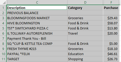
When analyzing our spending habits, it might be helpful to have a list of places we shopped and their corresponding categories. In this case, it isn't necessary to know when a purchase was made or the running balance. All we need is the description, category, and purchase price. By using a combination of hiding columns, copying only the visible data, and removing duplicate values, the data in this worksheet can be viewed in a very different way.
Available Files
The following files are available for download:
Hiding data in a worksheet
We will begin by hiding the data we don't need. When data is hidden, it has not been deleted or removed. It can be restored at any time.
We will be working in the March worksheet.
- Move to the March worksheet, if necessary.
- To select columns A and B, in the column headers,
Press & Drag columns A and B
- To hide columns A and B,
Right-Click the selected columns, Click Hide
Columns A and B are hidden. Column C is now the left-most column in the worksheet. The hidden columns have not been deleted and can be unhidden at any time.
Now let's hide the Type column, column E.
- To select column E, in the column headers,
Click column E
- To hide column E,
Right-Click the selected column, Click Hide
The Type column is hidden. We can see that the column headers go from D to F. There is also a dark line between columns D and F. The hidden columns are still selected even if we can't see them.
- Deselect the hidden columns.
We will finish by hiding the last two columns in the worksheet.
- To select columns G and H, in the column headers,
Press & Drag columns G and H
- To hide columns G and H,
Right-Click the selected columns, Click Hide
- Deselect the hidden columns.
With many of the columns hidden, our worksheet now shows simply the Description, Category, and Purchase for each transaction.
Copying visible data
Let's copy and paste this data into a new worksheet. When data has been hidden, it can still be copied and pasted. Sometimes that is beneficial and sometimes it isn't. There is an easy way to copy and paste only the visible data.
- To select all of the data in the March worksheet, on the keyboard, press:
Control key + A
When all of the data was selected, that included the hidden columns. If we were to copy and paste the current selection, the hidden columns would be pasted along with the visible data. We need to select, then copy, only the visible data.
- To open the Go To Special dialog box, on the Home tab,
Click
 , Click Go To Special...
 - To select only the visible cells, on the Home tab,
Click the Visible cells only radio button, Click

The selection changes slightly:

There is now a border around the hidden columns. This border appears as a heavy white line.
Any action we take will be applied to the visible cells. Let's see how this works by copying and pasting the contents of the visible cells.
- To copy the visible data, on the keyboard, press:
Control key + C
- To insert a new worksheet, at the bottom of the workbook,
Click

- To rename the new worksheet,
Double-Click the new worksheet name, type: Descriptions Enter key
- To paste the visible cells in the Descriptions worksheet, on the keyboard, press:
Control key + V
- To widen the columns, in the column headers,
Press & Drag columns A through C, Double-Click between the column A header and the column B header
- Deselect the columns.
- Save the workbook.
With the values copied into a new worksheet, let's move on to removing duplicate data.

