Utilizing special cell formats

When data is entered into a spreadsheet, by default, the General format is applied. The General format left aligns text and right aligns numbers. There are other formats that can be applied, including but not limited to Number, Currency, and Date. Occasionally there is data that doesn't fit one of the predefined formats. In these cases, we can use a Special format or even create a Custom format. 

Applying a Special cell format 

With the address information separated into four columns, it may be more evident that the zip codes aren't quite right. Some of them are only four digits. A standard United States zip code uses five numbers. In many parts of the eastern U.S., the zip codes start with a zero (0). When the address data was separated and the zip codes were moved to column K, Excel treated them as numbers. Excel doesn't allow numbers to start with zero (0) and automatically removed that digit. Although zip codes are technically numbers, they aren't used in mathematical functions and should be treated as text. Excel has a special format just for zip codes. By applying this format, the leading zero (0) will be returned to the appropriate zip codes. 

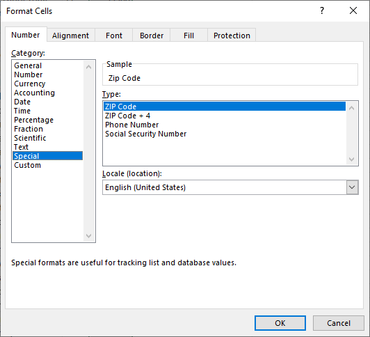
The ZIP Code format is in the Special category.

The Format Cells dialog box now shows the Special category:

Because we are using English (United States) as our location, we see four special formats. (Other languages and locations may have more or fewer special formats available.) These formats, ZIP Code, ZIP Code + 4, Phone Number, and Social Security Number, are all numbers that are treated as text. 

The leading zeros have been returned to the appropriate zip codes. 

Creating a Custom cell format

If there isn't a predefined cell format for the data, a Custom format can be created and applied. Custom formats can be used for many types of formatting including standard text, decimal point alignment, leading zeros, and date formatting. 

The Employee ID numbers in column A are all five digits. Let's update this so that there is a hyphen between the second and third digits. We will create a Custom cell format and apply it to all of column A. When finished, the ID numbers will look like this: 34-567.

There are several examples of custom cell formats. However, none of these fit our purpose. We will create our own custom format. To do this, we will use zeros as placeholders for numbers and will add the hyphen between the second and third digits. The format will look like this: 00-000. 

The custom format will be created in the Type field of the dialog box. If there is currently text in this field, it will need to be removed.

The Employee ID numbers are now formatted with a hyphen between the second and third digits. Because the formatting was applied to the entire column, if a new employee is added, the ID number will automatically be formatted that way. The person inputting the information will not have to type the hyphen.