Excel easily works with data created in different applications, including Access and other database tools, text files, and online sources. As long as this external data is saved in a format Excel can recognize, it can be imported into Excel where it can be manipulated and formatted.
Available Files
The following files are available for download:
Opening the source data
A common way to share data is by saving it in an unformatted text file with each field of text separated by a delimiter such as a comma or tab. A delimited text file has a consistent structure for each record and each record is preceded by a return.
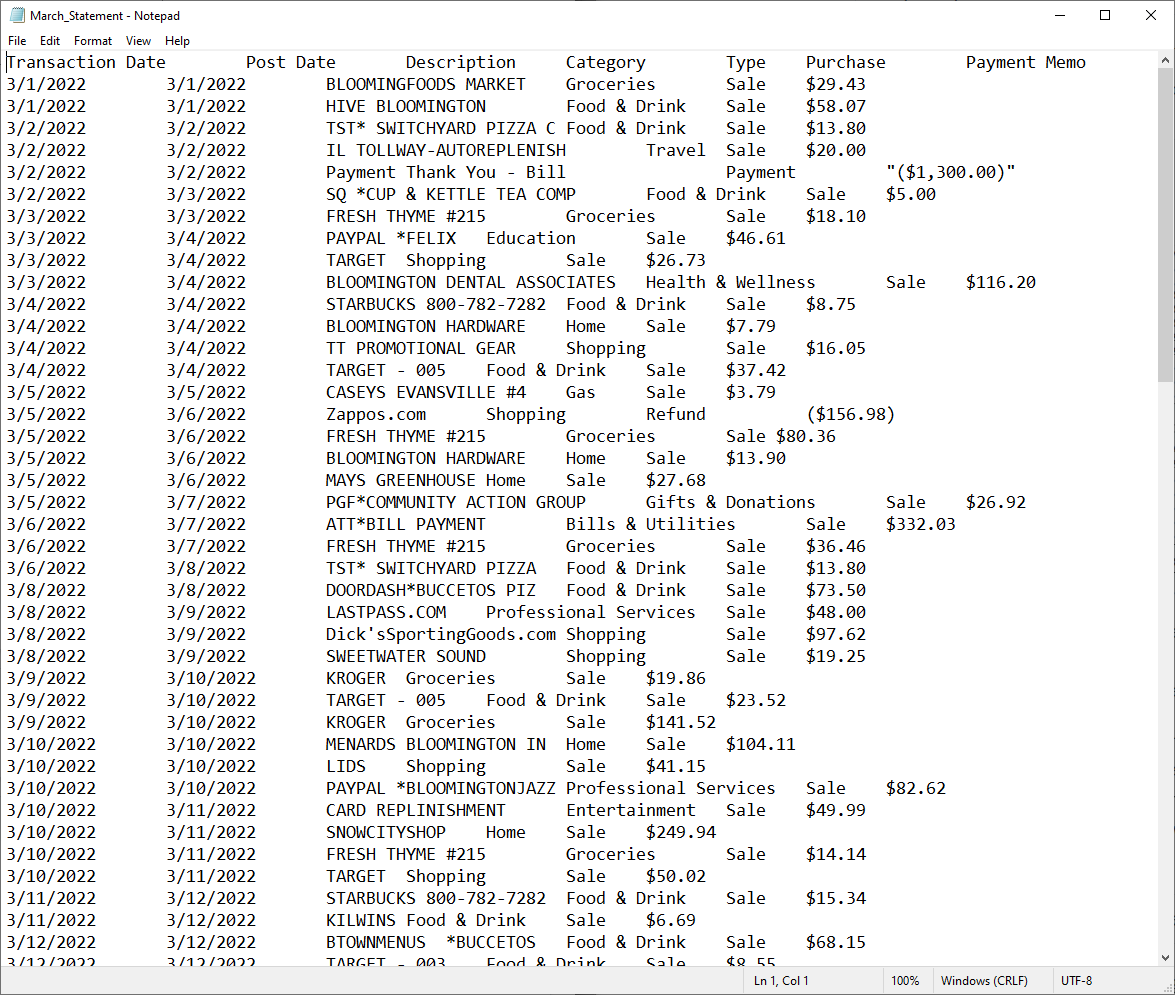
We are going to be working with a text file that contains a credit card statement for the month of March. Before we import this file into Excel, take a moment to look at it in its text form.
- To open the file March_Statement.txt,
navigate to the stored exercise files, Double-ClickMarch_Statement.txt
The file opens in a text editor:

This is a tab-delimited text (.txt) file. Each entry of the statement is on its own line with each individual element separated by pressing the Tab key. When this data is brought into Excel, each entry will be in its own row and each element will go in its own cell.
There are two ways to bring this data into Excel. One option is to simply open the file in Excel. If we do this, it will retain its original file type, with the .txt extension. We can then save it as an Excel file, with the .xlsx extension. The other option is to import it as an external data range. This will create a connection between the original file and the Excel workbook. For today's purposes, we will open the file in Excel. The Text Import Wizard will help us do this.
- To close the March_Statement.txt file, in the text editor,
Click File, Click Exit
Let's return to Excel and begin opening the .txt file. By default, Excel will only look for Excel files (.xlsx). We will have to adjust the file type to access the .txt file.
- Open Excel, if necessary.
- To begin opening the file March_Statement.txt, in Excel,
Click File, Click Open
- To find the file March_Statement.txt,
navigate to the stored exercise files
- In Microsoft Excel for Windows, to change the file type, in the lower left corner of the Open dialog box,
Click
 , Click Text Files
We now see only the .txt files contained in this folder.
- To open the Text Import Wizard,
Double-ClickMarch_Statement.txt
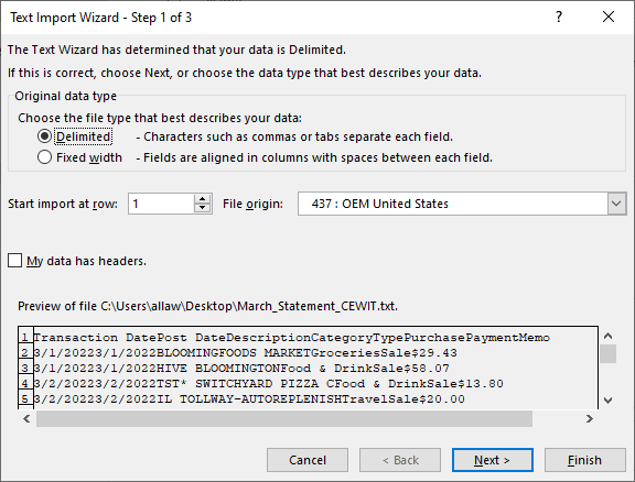
The Text Import Wizard opens:

The first step of the Text Import Wizard asks us to choose the data type, Delimited or Fixed Width. Our file is a delimited file. By default, the data will begin importing at row 1. In Microsoft Excel for Windows, there is a checkbox asking if the data has headers. At the bottom of the wizard, there is a preview of what the data will look like as we make changes.
- To confirm that the data has headers,
Click the My data has headers checkbox
- To move to step 2 of the wizard,
Click

- To move to step 2 of the wizard,
Click

In Step 2 of 3 of the Text Import Wizard, we can choose what type of delimiter is used in our data. This dataset is tab delimited.
- To deselect the Comma delimiter, if necessary,
Click the Comma checkbox
- To select the Tab delimiter, if necessary,
Click the Tab checkbox
- To move to step 3 of the wizard,
Click

The Text Import Wizard moves to Step 3. Here we are given the option to apply data formats to the columns before they are placed in Excel. We won't do this today. We will accept the default values.
- To accept the changes and close the wizard,
Click

The data is now in Excel, however, it is still a .txt file. Before we work with this file, we will need to save it as an Excel file. Let's save it as MarchStatement.xlsx.
- To begin saving the workbook,
Click File, Click Save As
- Navigate to the location where the exercise files are stored.
- To change the file name, in the File name field,
Press & drag the current name, type: MarchStatement
- To change the type of file, in the Save as type field,
Click
 , Click Excel Workbook or Excel Workbook (.xlsx)
 - To save the workbook,
Click

Cleaning up the data
Now that the workbook has been saved as an Excel file, we can begin working with the data.
This is a fictional credit card for the month of March. Before we get too involved in cleaning and formatting the data, let's open another Excel workbook. This workbook has statements from January and February. These statements have been cleaned and formatted. We want our March statement to look the same. There is also a third worksheet, Spending, where spending for each month has been calculated.
- To open the file Monthly_Statements.xlsx,
navigate to the stored exercise files, Double-ClickMonthly_Statements.xlsx
This workbook contains two monthly statements: January and February. Each worksheet contains a credit card statement for the corresponding month. Each has eight columns. The Balance column (column H) is calculated using the previous balance in the second row. The dates are in short format and payments are shown as negative numbers.
Let's return to the March statement and begin cleaning and formatting.
- To move to the View tab, on the Ribbon,
Click the View tab
- To return to the MarchStatment workbook, on the right side of the View tab,
Click
 , Click MarchStatement
There are several things to be done to the data in the March statement to make it look like the January and February data. We will begin by widening the columns to fit the data.
- To select columns A through H, in the column headers,
Press & Drag from column A through column H
- To widen the columns, in the header row,
Double-Click between any two column headers
Each column is now as wide as it needs to be to fit the data.
Let's format the column headings to be bold font. We'll select all of row 1 and apply the bold formatting.
- To select all of the contents of row 1, in the row headers,
Click row 1
- To make the column headings bold, on the Home tab,
Click

We need to change the format of the negative numbers in column G. They should include a negative symbol (-) and be in black font.
- To select column G, in the header row,
Click the column G header
- To open the Format Cells dialog box,
Right-Click the selected column, Click Format Cells...
- To select the Currency category, in the Category area,
Click Currency
- To change the format of negative numbers, in the Negative numbers area, if necessary,
Click -$1,234.10
- To accept this format, in the dialog box,
Click

- To deselect the selected cells,
Click in another cell
Now let's remove a column and add a row to the worksheet. The Memo column is unnecessary and we need a new row to hold the previous balance.
- To select the Memo column, in the header row,
Click the column H header
- To delete the column, on the keyboard, press:
Delete key
- Deselect the selected column.
- To select row 2, in the row headers,
Click row 2
- To insert a row above row 2,
Right-Click row 2, Click Insert
- Deselect the selected row.
- To add the description,
Click in cell C2, type: PREVIOUS BALANCE
The final change we need to make to the March worksheet is freezing the top two rows of data. When rows are frozen in Excel, they will remain at the top of the worksheet as we scroll down through the data. (Columns can also be frozen.) When freezing more than one row, the active cell should be in the row beneath the rows to be frozen.
- To make cell A3 the active cell,
Click in cell A3
- To move to the View tab, on the Ribbon,
Click the View tab
- To freeze row 1 and row 2, on the View tab,
Click
 , Click Freeze Panes
NOTE for MacOS users: In Microsoft Excel for MacOS, it is only necessary to click the Freeze Panes button one time.
The gridline between row 2 and row 3 is now darker and thicker indicating the above rows are frozen.
- To see how the frozen rows work, using the mouse,
scroll down
- To save the workbook, on the keyboard, press:
Control key + S
Now that the March statement looks similar to the previous statements, we're ready to move on to working across worksheets and analyzing the data.

