Let's create a pivot table that will show us information about donations (number, total, and average) based on donation date and campus. We will base this pivot table on the AlumniDonors worksheet.
Available Files
The following files are available for download:
- To move to the AlumniDonors worksheet, if necessary, at the bottom of the Excel window,
Click the AlumniDonors tab
- To begin creating the pivot table, on the Insert tab,
Click

- To place the pivot table in a new worksheet, in the dialog box,
Click

- To name the pivot table worksheet,
Double-Click the new worksheet tab, type: DonationsByDate Enter key
We want to see three types of information about the donation amounts: the total number, total amount, and average amount. To accomplish this, we will add the Donation Amount field to the pivot table Values area three times. By default, Excel will sum the donation amounts and provide the total amount of donations. We will use the Value Field Settings dialog box to change the calculation for the other two occurrences of the field to show the total number and average amount.
- To add the Donation Amount field to the Values area,
Press & Drag the Donation Amount field to the Values area
- Add the Donation Amount field to the Values area two more times.
- To select the first Donation Amount field, in the pivot table,
Click cell A3
- To open the Value Field Settings dialog box, in the PivotTable Analyze tab of the ribbon,
Click

- To change the calculation, in the "Summarize value field by" area,
Click Count, Click

With the first Donation Amount field now showing the number of donations, we will use the same process to change the second field to show the average amount.
- To select the first Donation Amount field, in the pivot table,
Click cell B3
- To open the Value Field Settings dialog box, in the PivotTable Analyze tab of the ribbon,
Click

- To change the calculation, in the "Summarize value field by" area,
Click Average, Click

With the three value fields set up, let's take a moment to format them and make them easier to understand. We'll change the names of the fields, format two of the fields as currency, and remove any decimal places.
- To change the name of the Count of Donation Amount field,
Click cell A3, type: Number of Donations
- To change the name of the Average of Donation Amount2 field,
Click cell B3, type: Average Donation
- To change the name of the Sum of Donation Amount3 field,
Click cell C3, type: Total Donations
- To select the two fields,
Press & drag cells B4:C4
- To open the Format Cells dialog box,
Right-Click the selected cells, Click Format Cells...
- To choose the Currency category, in the Format Cells dialog box,
Click Currency
- To remove the decimal places, in the Decimal places area,
Press & drag the current amount, type: 0
- To close the dialog box,
Click

With the value fields formatted correctly, we can add the remaining fields to the pivot table. We want to analyze the donation data based on donation date and campus. We will add both of these fields to the Rows area.
Grouping by date in a pivot table
When working with Microsoft Excel, dates will automatically be grouped when added to the pivot table. Depending on the format of the dates in the source data, Excel may add quarter, month, or year groupings to the pivot table. If the dates aren't in the format we want, it is easy to modify them.
- To add the Donation Date field to the Rows area,
Press & drag the Donation Date field to the Rows area
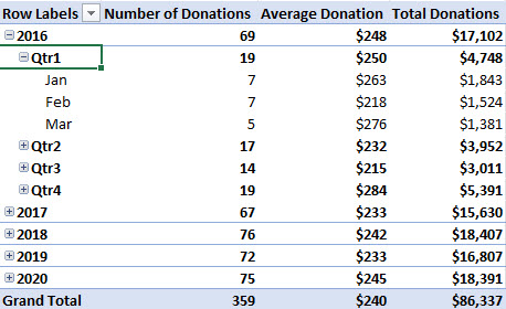
When the Donation Date field is added to the pivot table, Excel automatically groups the dates by years and quarters. These groups appear in the Rows area of the field list.

The pivot table currently shows only the years.

The quarters are contained within each year. These groups can be expanded and collapsed to show more or less detail.
- To expand the 2016 entry, in the pivot table,
Click

The 2016 entry expands and we now see the four quarters of the year.
- To expand the Qtr1 field, in the pivot table,
Click

The Qtr1 entry expands and we can see the donation information for the months within the quarter.

If the default groupings, years and quarters, aren't necessary or helpful, they can be removed or changed. Let's remove the quarters group and add a group to show us individual days. The steps for achieving this are different for Windows and macOs users. Follow the appropriate instructions below.
- To open the Grouping dialog box, on the PivotTable Analyze tab of the ribbon,
Click

NOTE: In Microsoft Excel for macOS, it may be necessary to Click  to see
 ![]() .
.
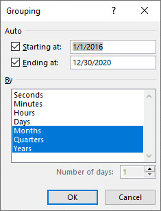
The Grouping dialog box opens:

In this dialog box, we can set the starting and ending values (in this case the values are dates). There are several date-related groups including Seconds, Minutes, Hours, Days, Months, Quarters, and Years. The Months, Quarters, and Years groups are selected.
- To remove the Quarters group, in the Grouping dialog box,
Click Quarters
- To add the Days group, in the Grouping dialog box,
Click Days
- To accept these changes and close the Grouping dialog box,
Click

- To add the Days group, in the Grouping dialog box,
Click Days
To add other groups, we will need to press & hold the Command key on the keyboard while selecting the groups with the mouse.
- To select the Months group, on the keyboard, press & hold:
Command key, Click Months
- To select the Years group, on the keyboard, press & hold:
Command key, Click Years
- To accept these changes and close the Grouping dialog box,
Click

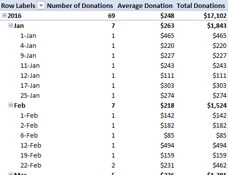
The pivot table changes and now shows us individual days when donations were made.

By default, all of the fields have been expanded. Before we move on, let's collapse them.
- To collapse all of the fields, in the pivot table,
Right-Click cell A4, Point to Expand/Collapse, Click Collapse Entire Field
The pivot table now shows the donation data by year.

- To save the workbook, on the keyboard, press:
Control key + S

